Workshop 5: Introduction to Bayesian models Murray Logan April 9, - PDF document

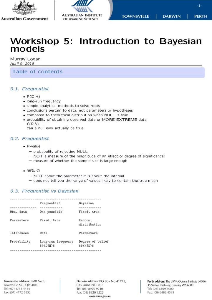
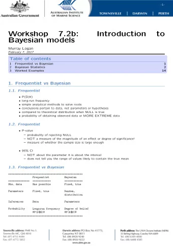
-1- Workshop 5: Introduction to Bayesian models Murray Logan April 9, 2016 Table of contents 0.1. Frequentist • P(D|H) • long-run frequency • simple analytical methods to solve roots • conclusions pertain to data, not parameters or hypotheses • compared to theoretical distribution when NULL is true • probability of obtaining observed data or MORE EXTREME data P ( D | H ) can a null ever actually be true 0.2. Frequentist • P-value – probabulity of rejecting NULL – NOT a measure of the magnitude of an effect or degree of significance! – measure of whether the sample size is large enough • 95% CI – NOT about the parameter it is about the interval – does not tell you the range of values likely to contain the true mean 0.3. Frequentist vs Bayesian ------------------------------------------------- Frequentist Bayesian -------------- ------------ ------------ Obs. data One possible Fixed, true Parameters Fixed, true Random, distribution Inferences Data Parameters Probability Long-run frequency Degree of belief $P(D|H)$ $P(H|D)$ -------------------------------------------------

-2- 0.4. Frequentist vs Bayesian 250 200 ● ● ● ● ● ● ● ● ● ● 150 100 50 0 2 4 6 8 10 x 250 ● ● 200 ● ● 150 ● ● ● ● ● 100 ● 50 0 2 4 6 8 10 x ● 250 ● ● ● ● ● ● ● 200 ● ● ● ● ● ● ● ● ● ● ● ● ● ● ● ● ● ● ● ● ● ● ● ● ● ● ● ● ● ● ● ● ● ● ● ● ● ● 150 ● ● ● ● ● ● ● ● ● ● ● ● ● ● ● ● ● ● ● ● ● ● ● ● ● ● ● ● ● ● 100 ● ● ● ● ● ● ● ● ● ● ● ● ● ● ● ● ● ● ● ● ● 50 ● 0 2 4 6 8 10 x n: 10 Slope: -0.1022 t: -2.3252 p: 0.0485 n: 10 Slope: -10.2318 t: -2.2115 p: 0.0579 n: 100 Slope: -10.4713 t: -6.6457 p: 1.7101362 Œ 10-9

-3- 0.5. Frequentist vs Bayesian 250 200 ● ● ● ● ● ● ● ● ● ● 150 100 50 0 2 4 6 8 10 x 250 ● ● 200 ● ● 150 ● ● ● ● ● 100 ● 50 0 2 4 6 8 10 x Population A Population B Percentage change 0.46 45.46 Prob. >5% decline 0 0.86 0.6. Bayesian 0.6.1. Bayes rule P ( H | D ) = P ( D | H ) × P ( H ) P ( D ) posterior belief ( probability ) = likelihood × prior probability normalizing constant 0.7. Bayesian

-4- 0.7.1. Bayes rule P ( H | D ) = P ( D | H ) × P ( H ) P ( D ) posterior belief ( probability ) = likelihood × prior probability normalizing constant The normalizing constant is required for probability - turn a frequency distribution into a probability distribution 0.8. Estimation: OLS 0.9. Estimation: Likelihood P ( D | H )

-5- 0.10. Bayesian • conclusions pertain to hypotheses • computationally robust (sample size,balance,collinearity) • inferential flexibility - derive any number of inferences 0.11. Bayesian • subjectivity? • intractable P ( H | D ) = P ( D | H ) × P ( H ) P ( D ) P ( D ) - probability of data from all possible hypotheses 0.12. MCMC sampling Marchov Chain Monte Carlo sampling • draw samples proportional to likelihood <ul> <li>two parameters $\alpha$ and $\beta$</li> <li>infinitely vague priors - posterior likelihood only</li> <li>likelihood multivariate normal</li>

-6- 0.13. MCMC sampling Marchov Chain Monte Carlo sampling • draw samples proportional to likelihood <ul> <li>two parameters $\alpha$ and $\beta$</li> <li>infinitely vague priors - posterior likelihood only</li> <li>likelihood multivariate normal</li> 0.14. MCMC sampling Marchov Chain Monte Carlo sampling

-7- • draw samples proportional to likelihood 0.15. MCMC sampling Marchov Chain Monte Carlo sampling

-8- • chain of samples 0.16. MCMC sampling Marchov Chain Monte Carlo sampling

-9- • 1000 samples 0.17. MCMC sampling Marchov Chain Monte Carlo sampling

-10- • 10,000 samples 0.18. MCMC sampling Marchov Chain Monte Carlo sampling • Aim: samples reflect posterior frequency distribution • samples used to construct posterior prob. dist. • the sharper the multidimensional “features” - more samples • chain should have traversed entire posterior • inital location should not influence 0.19. MCMC diagnostics

-11- 0.19.1. Trace plots 0.20. MCMC diagnostics 0.20.1. Autocorrelation • Summary stats on non-independent values are biased

-12- • Thinning factor = 1 0.21. MCMC diagnostics 0.21.1. Autocorrelation • Summary stats on non-independent values are biased

-13- • Thinning factor = 10 0.22. MCMC diagnostics 0.22.1. Autocorrelation • Summary stats on non-independent values are biased

-14- • Thinning factor = 10, n=10,000 0.23. MCMC diagnostics

-15- 0.23.1. Plot of Distributions 0.24. Native options in R • MCMCpack • MCMCglmm 0.25. JAGS/BUGS • WinBUGS - object pascal – made Bayesian analyses ‘available’ to masses – models mirror written definitions – very slow • JAGS - c++ – same declarative language – much faster 0.26. JAGS/BUGS • stand along application • file input

-16- – model declaration – data as a list • R2jags - interface from R 0.27. JAGS/BUGS ϵ ∼ N (0, σ 2 ) • y i = β 0 + β 1 x i + ϵ i • y i ∼ N ( β 0 + β 1 x i , σ 2 ) • y i ∼ N ( β 0 + β 1 x i , τ ) - τ is precision ( 1 σ 2 ) • y i ∼ N ( µ i , τ ) µ i = β 0 + β 1 x i – β 0 ∼ N (0, 0.000001) – β 1 ∼ N (0, 0.000001) 1 – τ = σ 2 – σ ∼ Uniform (0, 100) 0.28. JAGS/BUGS 0.28.1. Define the model > modelString=" + model { + #Likelihood + for (i in 1:n) { + y[i]~dnorm(mu[i],tau) + mu[i] <- beta0+beta1*x[i] + } + + #Priors + beta0 ~ dnorm (0,1.0E-6) + beta1 ~ dnorm(0,1.0E-6) + tau <- 1 / (sigma * sigma) + sigma~dunif(0,100) + } + " 1 y i ∼ N ( µ i , τ ) µ i = β 0 + β 1 x i β 0 ∼ N (0, 0.000001) β 1 ∼ N (0, 0.000001) τ = σ 2 σ ∼ Uniform (0, 100) > writeLines(modelString,con="BUGSscripts/regression.txt") Error in file(con, "w"): cannot open the connection 0.29. JAGS/BUGS 0.29.1. Create the data list Y X 3 0 2.5 1 6 2 5.5 3 9 4 8.6 5 12 6

-17- 0.30. JAGS/BUGS 0.30.1. Create the data list Y X 1 3.0 0 2 2.5 1 3 6.0 2 4 5.5 3 5 9.0 4 6 8.6 5 7 12.0 6 > data.list <- with(DATA, + list(y=Y, + x=X,n=nrow(DATA)) + ) > data.list $y [1] 3.0 2.5 6.0 5.5 9.0 8.6 12.0 $x [1] 0 1 2 3 4 5 6 $n [1] 7 0.31. JAGS/BUGS 0.31.1. Define the chain parameters > #params <- c("beta0","beta1","sigma") > #burnInSteps = 2000 > #nChains = 3 > #numSavedSteps = 50000 > #thinSteps = 1 > #nIter = ceiling((numSavedSteps * thinSteps)/nChains) 0.32. JAGS/BUGS 0.32.1. Perform MCMC sampling > library(R2jags)