Work Sheet 1: Scales and Aggregation Scales Assign the measure - PDF document

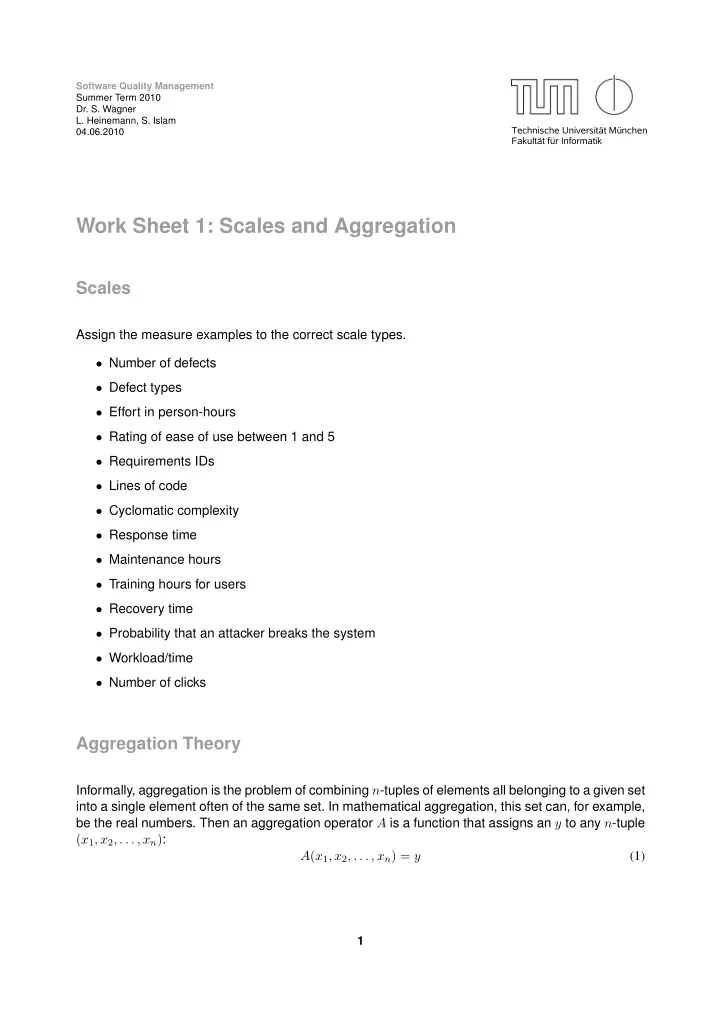
Software Quality Management Summer Term 2010 Dr. S. Wagner L. Heinemann, S. Islam Technische Universität München 04.06.2010 Fakultät für Informatik Work Sheet 1: Scales and Aggregation Scales Assign the measure examples to the correct scale types. • Number of defects • Defect types • Effort in person-hours • Rating of ease of use between 1 and 5 • Requirements IDs • Lines of code • Cyclomatic complexity • Response time • Maintenance hours • Training hours for users • Recovery time • Probability that an attacker breaks the system • Workload/time • Number of clicks Aggregation Theory Informally, aggregation is the problem of combining n -tuples of elements all belonging to a given set into a single element often of the same set. In mathematical aggregation, this set can, for example, be the real numbers. Then an aggregation operator A is a function that assigns an y to any n -tuple ( x 1 , x 2 , . . . , x n ) : A ( x 1 , x 2 , . . . , x n ) = y (1) 1

The literature defines additional properties that are requirements for a function to be called an aggregation operator . However, these properties are not all compatible. Yet, there seem to exist some undisputed properties that must be satisfied. For simplification, the sets that aggregation operators are based on are usually defined as [0 , 1] , i.e., the real numbers between 0 and 1. However, other sets can be used and by normalisation to this set it can be shown that the function is an aggregation operator. Additionally, the following must hold: A ( x ) = x identity when unary (2) A (0 , . . . , 0) = 0 ∧ A (1 , . . . , 1) = 1 boundary conditions (3) ∀ x i , y i : x i ≤ y i ⇒ A ( x 1 , . . . , x n ) ≤ A ( y 1 , . . . , y n ) monotonicity (4) The first condition obviously only is relevant for unary aggregation operators, i.e., the tuple that needs to be aggregated only has a single element. Then we expect the result of the aggregation to be that element. The boundary condition cover the extreme cases of the aggregation operator. With only minimal input there must be the minimum output and vice-versa. Finally, we expect that an aggregation operator is monotone. If all values stayed the same or increased we want the aggregation result also to increase or at least stay the same. Apart from these three conditions, there is a variety of further properties that an aggregation opera- tor can have. We only introduce three more that are relevant for aggregation operators of software measures. The first condition that introduces a very basic classification of aggregation operators is associati- vity . An operator is associative if the results keep the same no matter in what packages the results are computed. This has interesting effects on the implementation of the operator as associative operators are far easier to compute. Formally for an associative aggregation operator A a the follo- wing holds: A a ( x 1 , x 2 , x 3 ) = A a ( A a ( x 1 , x 2 ) , x 3 ) = A a ( x 1 , A a ( x 2 , x 3 )) (5) The next interesting property is symmetry . This is also known as commutativity or anonymity . If an aggregation operator is symmetrical, the order of the input arguments has no influence on the results. For every permutation σ of 1 , 2 , . . . , n the operator A s must satisfy: A s ( x σ (1) , x σ (2) , . . . , x σ ( n ) = A s ( x 1 , x 2 , . . . , x n ) (6) The last property we look at because it holds for some of the operators relevant for software mea- sures is idempotence . It is also known as unanimity or agreement . Idempotence means that if the input consists of only equal values, it is expected that the result is also this value. A i ( x, x, . . . , x ) = x (7) Aggregation Operators 2

Grouping A very high level aggregation is to define a set of groups, probably with a name each, and assign the inputs to the groups. This allows a very quick comprehension and easy communication about the results. However, the information loss is rather large. Rescaling. An often used technique to be able to overlook the large amount of information provided by various metrics is to change the scale type by grouping the individual values. This is usually done from higher scales such as ratio scales to ordinal or nominal scales. For example, we could define a certain threshold value. Above the group is red , below it is green . This is useful for all purposes apart from trend analysis where it can be applied only in a few cases. It is not idempotent in general and it depends on the specifics of the rescaling whether it is symmetrical. Cluster Analysis. Another, more sophisticated way, to find regularities in the input is cluster ana- lysis. It does basically the same thing as the rescaling described above but with finding the groups using clustering algorithms. The K-means [ ? ] algorithm is a common example of such algorithms. It works with the idea that the input are points scattered over a plain and there is a distance measure that can express the space between the points. The algorithms then works out which points should fall into the same cluster. This aggregator is not associative and not idempotent. Central Tendency The central tendency describes what colloquially is called the average. There are several aggrega- tion operators that can be used for determining this average of an input. They depend on the scale type of the measures the are aggregating. All of them are not associative but idempotent. Mode. The mode is the only way for analysing the central tendency for measures in a nominal sca- le. Intuitively, it gives the value that occurs most often in the input. Hence, for inputs with more than one maximum, the mode is not uniquely defined. If the result is then defined by the sequence of inputs, the mode is not symmetrical. The mode is useful for assessing the current state of a system and for comparisons w.r.t. measures in a nominal scale. For n 1 , . . . , n k being the frequencies of the input values, the mode M m is defined as M m ( x 1 , . . . , x k ) = x j ⇔ n j = max ( n 1 , . . . , n k ) . (8) Median. The median is the central tendency for metrics in an ordinal scale. An ordinal scale allows to enforce an order on the values and hence a value that is in the middle can be found. The median ensures that at most 50% of the values are smaller and at most 50% are greater or equal. The median is useful for assessing the current state and comparisons. The median M 0 . 5 is defined as � x (( n +1) / 2) if n is odd M 0 . 5 ( x 1 , . . . , x k ) = (9) 1 2 ( x ( n/ 2) + x ( n/ 2+1) otherwise The median of measures in ordinal scale, the division by 2 is not possible. Hence, in this case there are two medians. Mean. For measures in interval, ratio, or absolute scale, the mean value is defined. There are mainly three instances of means: arithmetic, geometric, and harmonic mean. The arithmetic mean is what usually is considered as average. It can be used for assessing the current state, predictions and comparisons. The arithmetic mean M a is defined as follows: n M a ( x 1 , . . . , x n ) = 1 � x i (10) n i =1 3