Why Copulas Have Been Successful From 1-D to Multi-D in Many - PowerPoint PPT Presentation
Introduction How to Represent . . . Case of 1-D . . . Multi-D Case Why Copulas Have Been Successful From 1-D to Multi-D in Many Practical Applications: What is an Algorithm: . . . A Theoretical Explanation What Is An Algorithm: . . . Based
Introduction How to Represent . . . Case of 1-D . . . Multi-D Case Why Copulas Have Been Successful From 1-D to Multi-D in Many Practical Applications: What is an Algorithm: . . . A Theoretical Explanation What Is An Algorithm: . . . Based on Computational Efficiency Computationally . . . Conclusions Vladik Kreinovich 1 , Hung T. Nguyen 2 , 3 , Home Page Songsak Sriboonchitta 3 , and Olga Kosheleva 4 Title Page 1 Department of Computer Science, 4 Department of Teacher Education ◭◭ ◮◮ University of Texas at El Paso, El Paso, Texas 79968, USA ◭ ◮ vladik@utep.edu, olgak@utep.edu, 2 Department of Mathematical Sciences, New Mexico State University Page 1 of 18 Las Cruces, New Mexico 88003, USA, hunguyen@nmsu.edu 3 Faculty of Economics, Chiang Mai University Go Back Chiang Mai, Thailand, songsakecon@gmail.com Full Screen Close Quit
Introduction How to Represent . . . 1. Introduction Case of 1-D . . . • In many practical problems, we deal with joint distri- Multi-D Case butions of several quantities (multi-D distributions). From 1-D to Multi-D What is an Algorithm: . . . • There are many different ways to represent such a dis- What Is An Algorithm: . . . tribution in a computer. Computationally . . . • In many practical applications, it turns out to be ben- Conclusions eficial to use a representation in which we store: Home Page • the marginal distributions (that describe the distri- Title Page bution of each quantity) and ◭◭ ◮◮ • a copula (that describe the relation between differ- ◭ ◮ ent quantities; definitions are given below). Page 2 of 18 • While this representation is, in many cases, empirically successful, this empirical success is largely a mystery. Go Back • We explain this success by showing that the copula Full Screen representation is the most computationally efficient. Close Quit
Introduction How to Represent . . . 2. How to Represent Probability Distributions: Case of 1-D . . . Idea Multi-D Case • The main purpose of knowledge is to make decisions. From 1-D to Multi-D What is an Algorithm: . . . • According to decision theory, a consistent decision What Is An Algorithm: . . . comes from the following: Computationally . . . • we assign a numerical value u (called utility ) to each Conclusions possible consequence, and then Home Page • we select a decision for which the expected value Title Page E [ u ] of utility is the largest possible. ◭◭ ◮◮ • We should select a representation that facilitates deci- ◭ ◮ sion making. Page 3 of 18 • So, we need a representation that allows us to compute Go Back the expected utility as efficiently as possible. Full Screen Close Quit
Introduction How to Represent . . . 3. Case of 1-D Probability Distributions Case of 1-D . . . • Example – transportation: we want to get from point Multi-D Case A to point B as fact as possible. From 1-D to Multi-D What is an Algorithm: . . . • Often, a small increase in travel time x leads to a small What Is An Algorithm: . . . decrease in utility u ( x ): u ( x ) is smooth. Computationally . . . • Usually, we can predict x with some accuracy, so the Conclusions actual x is in a small vicinity of the predicted value x 0 . Home Page • In this vicinity: Title Page u ( x ) = u ( x 0 )+ u ′ ( x 0 ) · ( x − x 0 )+1 ◭◭ ◮◮ 2 · u ′′ ( x 0 ) · ( x − x 0 ) 2 + . . . , so ◭ ◮ E [ u ] = u ( x 0 )+ u ′ ( x 0 ) · E [ x − x 0 ]+1 2 · u ′′ ( x 0 ) · E [( x − x 0 ) 2 ]+ . . . Page 4 of 18 Go Back • So, to compute E [ u ], it is sufficient to know the first few moments of the probability distribution. Full Screen Close Quit
Introduction How to Represent . . . 4. 1-D Distributions (cont-d) Case of 1-D . . . • Sometimes, e.g., if we are driving to the airport to take Multi-D Case a flight – a small delay can make us miss a flight. From 1-D to Multi-D What is an Algorithm: . . . • In such situations, we have a threshold x t such that: What Is An Algorithm: . . . • the utility is high for x ≤ x t and Computationally . . . • low for x > x t . Conclusions Home Page • The difference between two high values is much smaller than between high and low values. Title Page • Thus, we can simply say that u = u + for x ≤ x t and ◭◭ ◮◮ u = u − < u + for x > x t . ◭ ◮ • In this case, E [ u ] = u − + ( u + − u − ) · F ( x t ), where Page 5 of 18 F ( x t ) = Prob( x ≤ x t ) is the probability that x ≤ x t . Go Back • So, to deal with situations of this type, we need to Full Screen know the cdf F ( x ). Close Quit
Introduction How to Represent . . . 5. 1-D Distributions: Conclusion Case of 1-D . . . • Our analysis shows that in the 1-D case, to compute Multi-D Case the expected utilities, we need to know: From 1-D to Multi-D What is an Algorithm: . . . • the cdf and What Is An Algorithm: . . . • the moments. Computationally . . . • Moments can be computed based on cdf, as Conclusions Home Page � ( x − x 0 ) k dF ( x ) . E [( x − x 0 ) k ] = Title Page ◭◭ ◮◮ • So, it is thus sufficient to have a cdf; hence: ◭ ◮ • the most appropriate way to represent a 1-D prob- ability distribution in the computer is Page 6 of 18 • to store the values of its cumulative distribution Go Back function F ( x ). Full Screen Close Quit
Introduction How to Represent . . . 6. Multi-D Case Case of 1-D . . . • When small changes in x i lead to small changes in Multi-D Case u ( x 1 , . . . , x n ), it’s enough to know first few moments. From 1-D to Multi-D What is an Algorithm: . . . • In the situations of the second type, we want all the What Is An Algorithm: . . . values not to exceed appropriate thresholds; e.g.: Computationally . . . • the travel time does not exceed T 0 , and Conclusions • the overall cost of all the tolls does not exceed C 0 . Home Page • So, it is desirable to know the following probabilities – Title Page that form the corresponding multi-D cdf: ◭◭ ◮◮ def F ( x 1 , . . . , x n ) = Prob( X 1 ≤ x 1 & . . . & X n ≤ x n ) . ◭ ◮ Page 7 of 18 • Hence, in the multi-D case, we need to compute both the moments and the multi-D cdf. Go Back • Since the moments can be computed based on the cdf, Full Screen it is thus sufficient to represent a cdf. Close Quit
Introduction How to Represent . . . 7. From 1-D to Multi-D Case of 1-D . . . • The above analysis of is appropriate when we acquire Multi-D Case all our knowledge about the probabilities in one step. From 1-D to Multi-D What is an Algorithm: . . . • However, often, first we are interested in each x i , so we What Is An Algorithm: . . . first learn the marginals F i ( x i ). Computationally . . . • Later, we become interested in the relation between Conclusions these x i , so we need the cdf F ( x 1 , . . . , x n ). Home Page • But storing F ( x 1 , . . . , x n ) and marginals wastes mem- Title Page ory: marginals can be reconstructed from F . ◭◭ ◮◮ • An alternative is to store a copula , i.e., a function ◭ ◮ C ( x 1 , . . . , x n ) s.t. Page 8 of 18 F ( x 1 , . . . , x n ) = C ( F 1 ( x 1 ) , . . . , F n ( x n )) . Go Back • Copula representation avoids memory waste, but is it optimal? is it the only optimal one? Full Screen • Let us formulate this question in precise terms. Close Quit
Introduction How to Represent . . . 8. What is an Algorithm: Reminder Case of 1-D . . . • We want to be able, given the marginals and the addi- Multi-D Case tional function(s), to reconstruct F ( x 1 , . . . , x n ). From 1-D to Multi-D What is an Algorithm: . . . • This reconstruction has to be done by a computer al- What Is An Algorithm: . . . gorithm , a sequence of steps, in each of which we: Computationally . . . • either apply some operation (+, − , sin, given func- Conclusions tion) to previously computed values, Home Page • or decide where to go further (or stop). Title Page • In computations, we can use inputs, previous compu- ◭◭ ◮◮ tation results, and constants (including ±∞ ). ◭ ◮ • We can also use NaN (undefined): if one of the inputs Page 9 of 18 is undefined, the result is also undefined. Go Back Full Screen Close Quit
Introduction How to Represent . . . 9. What Is An Algorithm: Definition Case of 1-D . . . • Let F be a finite list of functions f i ( z 1 , . . . , z n i ). Multi-D Case From 1-D to Multi-D • Let v 1 , . . . , v m be a finite list of real-valued variables What is an Algorithm: . . . called inputs . What Is An Algorithm: . . . • Let a 1 , . . . , a p be a finite list of real-valued variables Computationally . . . called auxiliary variables . Conclusions Home Page • Let r 1 , . . . , r q be real-valued variables; they will be called the results of the computations. Title Page • An algorithm A is a finite sequence of instructions ◭◭ ◮◮ I 1 , . . . , I N each of which has one of the following forms: ◭ ◮ • assignment: “ y ← y 1 ” or “ y ← f i ( y 1 , . . . , y n i ) ” ; Page 10 of 18 • branching: “go to I i ”; or “if y 1 ⊙ y 2 , then to I i else Go Back go to I j ” , where ⊙ is =, � =, < , > , ≤ , or ≥ ; Full Screen • “stop” . Close Quit
Recommend
More recommend
Explore More Topics
Stay informed with curated content and fresh updates.
