When are we committed to crossing critical (1.5 or 2 C) temperature - PowerPoint PPT Presentation
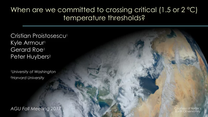
When are we committed to crossing critical (1.5 or 2 C) temperature thresholds? Cristian Proistosescu 1 Kyle Armour 1 Gerard Roe 1 Peter Huybers 2 1 University of Washington 2 Harvard University AGU Fall Meeting 2017 Courtesy of NASAs Earth
When are we committed to crossing critical (1.5 or 2 °C) temperature thresholds? Cristian Proistosescu 1 Kyle Armour 1 Gerard Roe 1 Peter Huybers 2 1 University of Washington 2 Harvard University AGU Fall Meeting 2017 Courtesy of NASA’s Earth Observatory
Two questions 1. When will we cross 1.5 or 2 °C global warming thresholds (e.g., following high or low emission scenarios) – subject to constraints from the observed global energy budget? 2. When will we be geophysically committed to crossing 1.5 or 2 °C global warming thresholds?
What do CMIP5 models say? CMIP5 projections (IPCC AR5) 2 °C
What do CMIP5 models say? § Models may not agree with observed CMIP5 projections (IPCC AR5) global warming and energy budget constraints § Models may not span full range of plausible future warming § Computationally expensive to run different emissions scenarios, so can’t ask questions like, when are we geophysically committed to 2 °C? 2 °C § Not clear which physical factors are contributing to uncertainty in projected warming
Our approach § Use a 2-layer ocean model (Held et al. 2010; radiative radiative + F + = � T u + response Armour 2017) that includes the essential physics forcing governing global-mean surface warming: Ocean heat uptake efficacy dT u upper ocean T u dt = � T u + F + "� ( T d � T u ) ( c u deep ocean T d dT d = � ( T u � T d ) ( dt = � ( T u � T d ) ( c d
Our approach § Use a 2-layer ocean model (Held et al. 2010; Global surface temperature response Armour 2017) that includes the essential physics to abrupt CO 2 quadrupling governing global-mean surface warming: Temperature change T (°C) 6 3 dT u dt = � T u + F + "� ( T d � T u ) ( c u 2 4 Slow warming on timescale of the dT d deep ocean dt = � ( T u � T d ) 1 ( c d 2 Fast warming on timescale of the surface 0 0 0 50 100 150 0 50 100 150 Year after CO 2 quadrupling
Our approach § Use a 2-layer ocean model (Held et al. 2010; Global surface temperature response Armour 2017) that includes the essential physics to abrupt CO 2 quadrupling governing global-mean surface warming: Temperature change T (°C) 6 3 dT u dt = � T u + F + "� ( T d � T u ) ( c u 2 4 dT d dt = � ( T u � T d ) 1 ( c d 2 0 0 0 50 100 150 0 50 100 150 Year after CO 2 quadrupling
Our approach § Use a 2-layer ocean model (Held et al. 2010; � ( Step 1: Draw priors of , , , and from fits + "� c u c d � T Armour 2017) that includes the essential physics of 2-layer model to CMIP5 model response to governing global-mean surface warming: CO 2 forcing (Geoffroy et al. 2013) dT u dt = � T u + F + "� ( T d � T u ) ( c u dT d dt = � ( T u � T d ) ( c d
Our approach § Use a 2-layer ocean model (Held et al. 2010; � ( Step 1: Draw priors of , , , and from fits + "� c u c d � T Armour 2017) that includes the essential physics of 2-layer model to CMIP5 model response to governing global-mean surface warming: CO 2 forcing (Geoffroy et al. 2013) Step 2: Drive model with timeseries of historical radiative forcing (Meinshausen et al. 2011), with priors drawn from forcing range in IPCC AR5 dT u dt = � T u + F + "� ( T d � T u ) ( c u dT d dt = � ( T u � T d ) ( c d
Our approach § Use a 2-layer ocean model (Held et al. 2010; � ( Step 1: Draw priors of , , , and from fits + "� c u c d � T Armour 2017) that includes the essential physics of 2-layer model to CMIP5 model response to governing global-mean surface warming: CO 2 forcing (Geoffroy et al. 2013) Step 2: Drive model with timeseries of historical radiative forcing (Meinshausen et al. 2011), with priors drawn from forcing range in IPCC AR5 dT u dt = � T u + F + "� ( T d � T u ) ( c u Step 3: Use Bayesian inference to estimate posterior parameters/forcings based on dT d observed warming and energy budget (see dt = � ( T u � T d ) ( c d also: Forest et al. 2002, 2006; Stott & Forest 2007) ⇥ T obs = 0.75 ± 0.2 °C (Otto et al. 2013; = 0.65 ± 0.27 Wm -2 − Q obs 2000-2009 relative to ⇥ 1860-1879) = F obs = 2.3 ± 1 Wm -2
Our approach � ( Step 1: Draw priors of , , , and from fits + "� c u c d � T of 2-layer model to CMIP5 model response to 2-layer model historical warming CO 2 forcing (Geoffroy et al. 2013) Temperature change [°C] Step 2: Drive model with timeseries of historical radiative forcing (Meinshausen et al. 2011), with priors drawn from forcing range in IPCC AR5 Step 3: Use Bayesian inference to estimate posterior parameters/forcings based on observed warming and energy budget (see also: Forest et al. 2002, 2006; Stott & Forest 2007) ⇥ T obs = 0.75 ± 0.2 °C (Otto et al. 2013; = 0.65 ± 0.27 Wm -2 − Q obs 2000-2009 relative to ⇥ 1860-1879) = Year F obs = 2.3 ± 1 Wm -2
Our approach � ( Step 1: Draw priors of , , , and from fits + "� c u c d � T of 2-layer model to CMIP5 model response to 2-layer model historical warming CO 2 forcing (Geoffroy et al. 2013) Temperature change [°C] Step 2: Drive model with timeseries of historical radiative forcing (Meinshausen et al. 2011), with priors drawn from forcing range in IPCC AR5 Step 3: Use Bayesian inference to estimate posterior parameters/forcings based on observed warming and energy budget (see also: Forest et al. 2002, 2006; Stott & Forest 2007) Step 4: Use the observationally-constrained parameter/forcing estimates to project warming, and committed warming, following RCP2.6 and RCP8.5 emissions scenarios Year
Our approach � ( Step 1: Draw priors of , , , and from fits + "� c u c d � T of 2-layer model to CMIP5 model response to 2-layer model projections CO 2 forcing (Geoffroy et al. 2013) Temperature change [°C] Step 2: Drive model with timeseries of historical radiative forcing (Meinshausen et al. 2011), with priors drawn from forcing range in IPCC AR5 Step 3: Use Bayesian inference to estimate posterior parameters/forcings based on observed warming and energy budget (see also: Forest et al. 2002, 2006; Stott & Forest 2007) Step 4: Use the observationally-constrained parameter/forcing estimates to project warming, and committed warming, following RCP2.6 and RCP8.5 emissions scenarios Year
Our approach � ( Step 1: Draw priors of , , , and from fits + "� c u c d � T of 2-layer model to CMIP5 model response to 2-layer model projections CO 2 forcing (Geoffroy et al. 2013) Temperature change [°C] Step 2: Drive model with timeseries of historical radiative forcing (Meinshausen et al. 2011), with priors drawn from forcing range in IPCC AR5 Step 3: Use Bayesian inference to estimate posterior parameters/forcings based on observed warming and energy budget (see also: Forest et al. 2002, 2006; Stott & Forest 2007) Step 4: Use the observationally-constrained parameter/forcing estimates to project warming, and committed warming, following RCP2.6 and RCP8.5 emissions scenarios Year
Our approach � ( Step 1: Draw priors of , , , and from fits + "� c u c d � T of 2-layer model to CMIP5 model response to 2-layer model projections CO 2 forcing (Geoffroy et al. 2013) Temperature change [°C] Step 2: Drive model with timeseries of historical radiative forcing (Meinshausen et al. 2011), with priors drawn from forcing range in IPCC AR5 Step 3: Use Bayesian inference to estimate posterior parameters/forcings based on observed warming and energy budget (see also: Forest et al. 2002, 2006; Stott & Forest 2007) Step 4: Use the observationally-constrained parameter/forcing estimates to project warming, and committed warming, following RCP2.6 and RCP8.5 emissions scenarios Year
Our approach 2-layer model projections CMIP5 projections (IPCC AR5) Temperature change [°C] Year
When are we going to cross 1.5 or 2 °C thresholds? 2-layer model projections Year at which 2 °C is crossed Temperature change [°C] Probability density [1/yr] Year Year
When are we going to cross 1.5 or 2 °C thresholds? 2-layer model projections Year at which 2 °C is crossed Temperature change [°C] Probability density [1/yr] Year Year Probability of crossing 2.0 °C along RCP 2.6 = 0.13
When are we going to cross 1.5 or 2 °C thresholds? 2-layer model projections Year at which 1.5 °C is crossed Temperature change [°C] Probability density [1/yr] Year Year Probability of crossing 1.5 °C along RCP 2.6 = 0.41
Zero-emissions climate commitment § How much more warming will occur given no further human influence on climate? § Constant atmospheric composition requires continued emissions; the climate commitment is better defined with respect to past emissions only 1.5 Constant composition IPCC AR4 models Global temperature change ( °C) This study 1.0 Zero emissions BERN2.5CC model 0.5 HadCM3LC model (Matthews and Weaver 2010) 0.0 1800 1900 2000 2100 2200 2300 Year
Recommend
More recommend
Explore More Topics
Stay informed with curated content and fresh updates.
