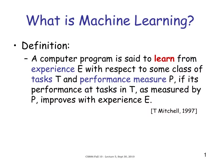
What is Machine Learning? Definition: A computer program is said to - PowerPoint PPT Presentation
What is Machine Learning? Definition: A computer program is said to learn from experience E with respect to some class of tasks T and performance measure P, if its performance at tasks in T, as measured by P, improves with experience E.
What is Machine Learning? • Definition: – A computer program is said to learn from experience E with respect to some class of tasks T and performance measure P, if its performance at tasks in T, as measured by P, improves with experience E. [T Mitchell, 1997] 1 CS886 Fall 10 - Lecture 5, Sept 30, 2010
Inductive learning (aka concept learning) • Induction: – Given a training set of examples of the form (x,f(x)) • x is the input, f(x) is the output – Return a function h that approximates f • h is called the hypothesis 2 CS886 Fall 10 - Lecture 5, Sept 30, 2010
Classification • Training set: Sky Humidity Wind Water Forecast EnjoySport Sunny Normal Strong Warm Same Yes Sunny High Strong Warm Same Yes Sunny High Strong Warm Change No Sunny High Strong Cool Change Yes f(x) x • Possible hypotheses: – h 1 : S=sunny ES=yes – h 2 : Wa=cool or F=same enjoySport 3 CS886 Fall 10 - Lecture 5, Sept 30, 2010
Regression • Find function h that fits f at instances x 4 CS886 Fall 10 - Lecture 5, Sept 30, 2010
Regression • Find function h that fits f at instances x h 1 h 2 5 CS886 Fall 10 - Lecture 5, Sept 30, 2010
Hypothesis Space • Hypothesis space H – Set of all hypotheses h that the learner may consider – Learning is a search through hypothesis space • Objective: – Find hypothesis that agrees with training examples – But what about unseen examples? 6 CS886 Fall 10 - Lecture 5, Sept 30, 2010
Generalization • A good hypothesis will generalize well (i.e. predict unseen examples correctly) • Usually… – Any hypothesis h found to approximate the target function f well over a sufficiently large set of training examples will also approximate the target function well over any unobserved examples 7 CS886 Fall 10 - Lecture 5, Sept 30, 2010
Inductive learning • Construct/adjust h to agree with f on training set • ( h is consistent if it agrees with f on all examples) • E.g., curve fitting: 8 CS886 Fall 10 - Lecture 5, Sept 30, 2010
Inductive learning • Construct/adjust h to agree with f on training set • ( h is consistent if it agrees with f on all examples) • E.g., curve fitting: 9 CS886 Fall 10 - Lecture 5, Sept 30, 2010
Inductive learning • Construct/adjust h to agree with f on training set • ( h is consistent if it agrees with f on all examples) • E.g., curve fitting: 10 CS886 Fall 10 - Lecture 5, Sept 30, 2010
Inductive learning • Construct/adjust h to agree with f on training set • ( h is consistent if it agrees with f on all examples) • E.g., curve fitting: 11 CS886 Fall 10 - Lecture 5, Sept 30, 2010
Inductive learning • Construct/adjust h to agree with f on training set • ( h is consistent if it agrees with f on all examples) • E.g., curve fitting: • Ockham’s razor: prefer the simplest hypothesis consistent with data 12 CS886 Fall 10 - Lecture 5, Sept 30, 2010
Performance of a learning algorithm • A learning algorithm is good if it produces a hypothesis that does a good job of predicting classifications of unseen examples • Verify performance with a test set 1. Collect a large set of examples 2. Divide into 2 disjoint sets: training set and test set 3. Learn hypothesis h with training set 4. Measure percentage of correctly classified examples by h in the test set 5. Repeat 2-4 for different randomly selected training sets of varying sizes 13 CS886 Fall 10 - Lecture 5, Sept 30, 2010
Learning curves Training set Overfitting! % correct Test set Size of hypothesis space 14 CS886 Fall 10 - Lecture 5, Sept 30, 2010
Overfitting • Definition : Given a hypothesis space H, a hypothesis h ∈ H is said to overfit the training data if there exists some alternative hypothesis h’ ∈ H such that h has smaller error than h’ over the training examples but h’ has smaller error than h over the entire distribution of instances • Overfitting has been found to decrease accuracy of many algorithms by 10-25% 15 CS886 Fall 10 - Lecture 5, Sept 30, 2010
Statistical Learning • View: we have uncertain knowledge of the world • Idea: learning simply reduces this uncertainty 16 CS886 Fall 10 - Lecture 5, Sept 30, 2010
Candy Example • Favorite candy sold in two flavors: – Lime (hugh) – Cherry (yum) • Same wrapper for both flavors • Sold in bags with different ratios: – 100% cherry – 75% cherry + 25% lime – 50% cherry + 50% lime – 25% cherry + 75% lime – 100% lime 17 CS886 Fall 10 - Lecture 5, Sept 30, 2010
Candy Example • You bought a bag of candy but don’t know its flavor ratio • After eating k candies: – What’s the flavor ratio of the bag? – What will be the flavor of the next candy? 18 CS886 Fall 10 - Lecture 5, Sept 30, 2010
Statistical Learning • Hypothesis H: probabilistic theory of the world – h 1 : 100% cherry – h 2 : 75% cherry + 25% lime – h 3 : 50% cherry + 50% lime – h 4 : 25% cherry + 75% lime – h 5 : 100% lime • Data D: evidence about the world – d 1 : 1 st candy is cherry – d 2 : 2 nd candy is lime – d 3 : 3 rd candy is lime – … 19 CS886 Fall 10 - Lecture 5, Sept 30, 2010
Bayesian Learning • Prior: Pr(H) • Likelihood: Pr(d|H) • Evidence: d = <d 1 ,d 2 ,…,d n > • Bayesian Learning amounts to computing the posterior using Bayes’ Theorem: Pr(H| d ) = k Pr( d |H)Pr(H) 20 CS886 Fall 10 - Lecture 5, Sept 30, 2010
Bayesian Prediction • Suppose we want to make a prediction about an unknown quantity X (i.e., the flavor of the next candy) • Pr(X| d ) = Σ i Pr(X| d ,h i )P(h i | d ) = Σ i Pr(X|h i )P(h i | d ) • Predictions are weighted averages of the predictions of the individual hypotheses • Hypotheses serve as “intermediaries” between raw data and prediction 21 CS886 Fall 10 - Lecture 5, Sept 30, 2010
Candy Example • Assume prior P(H) = <0.1, 0.2, 0.4, 0.2, 0.1> • Assume candies are i.i.d. (identically and independently distributed) – P( d |h) = Π j P(d j |h) • Suppose first 10 candies all taste lime: – P( d |h 5 ) = 1 10 = 1 – P( d |h 3 ) = 0.5 10 = 0.00097 – P( d |h 1 ) = 0 10 = 0 22 CS886 Fall 10 - Lecture 5, Sept 30, 2010
Posterior 23 CS886 Fall 10 - Lecture 5, Sept 30, 2010
Prediction Probability that next candy is lime 24 CS886 Fall 10 - Lecture 5, Sept 30, 2010
Bayesian Learning • Bayesian learning properties: – Optimal (i.e. given prior, no other prediction is correct more often than the Bayesian one) – No overfitting (prior can be used to penalize complex hypotheses) • There is a price to pay: – When hypothesis space is large Bayesian learning may be intractable – i.e. sum (or integral) over hypothesis often intractable • Solution: approximate Bayesian learning 25 CS886 Fall 10 - Lecture 5, Sept 30, 2010
Maximum a posteriori (MAP) • Idea: make prediction based on most probable hypothesis h MAP – h MAP = argmax hi P(h i | d ) – P(X| d ) ≈ P(X|h MAP ) • In contrast, Bayesian learning makes prediction based on all hypotheses weighted by their probability 26 CS886 Fall 10 - Lecture 5, Sept 30, 2010
Candy Example (MAP) • Prediction after – 1 lime: h MAP = h 3 , Pr(lime|h MAP ) = 0.5 – 2 limes: h MAP = h 4 , Pr(lime|h MAP ) = 0.75 – 3 limes: h MAP = h 5 , Pr(lime|h MAP ) = 1 – 4 limes: h MAP = h 5 , Pr(lime|h MAP ) = 1 – … • After only 3 limes, it correctly selects h 5 27 CS886 Fall 10 - Lecture 5, Sept 30, 2010
Candy Example (MAP) • But what if correct hypothesis is h 4 ? – h 4 : P(lime) = 0.75 and P(cherry) = 0.25 • After 3 limes – MAP incorrectly predicts h 5 – MAP yields P(lime|h MAP ) = 1 – Bayesian learning yields P(lime| d ) = 0.8 28 CS886 Fall 10 - Lecture 5, Sept 30, 2010
MAP properties • MAP prediction less accurate than Bayesian prediction since it relies only on one hypothesis h MAP • But MAP and Bayesian predictions converge as data increases • No overfitting (prior can be used to penalize complex hypotheses) • Finding h MAP may be intractable: – h MAP = argmax P(h| d ) – Optimization may be difficult 29 CS886 Fall 10 - Lecture 5, Sept 30, 2010
MAP computation • Optimization: – h MAP = argmax h P(h| d ) = argmax h P(h) P( d |h) = argmax h P(h) Π i P(d i |h) • Product induces non-linear optimization • Take the log to linearize optimization – h MAP = argmax h log P(h) + Σ i log P(d i |h) 30 CS886 Fall 10 - Lecture 5, Sept 30, 2010
Maximum Likelihood (ML) • Idea: simplify MAP by assuming uniform prior (i.e., P(h i ) = P(h j ) ∀ i,j) – h MAP = argmax h P(h) P( d |h) – h ML = argmax h P( d |h) • Make prediction based on h ML only: – P(X| d ) ≈ P(X|h ML ) 31 CS886 Fall 10 - Lecture 5, Sept 30, 2010
Candy Example (ML) • Prediction after – 1 lime: h ML = h 5 , Pr(lime|h ML ) = 1 – 2 limes: h ML = h 5 , Pr(lime|h ML ) = 1 – … • Frequentist: “objective” prediction since it relies only on the data (i.e., no prior) • Bayesian: prediction based on data and uniform prior (since no prior ≡ uniform prior) 32 CS886 Fall 10 - Lecture 5, Sept 30, 2010
Recommend
More recommend
Explore More Topics
Stay informed with curated content and fresh updates.


