Video denoising via Bayesian modeling of patches Pablo Arias joint - PowerPoint PPT Presentation
Video denoising via Bayesian modeling of patches Pablo Arias joint work with Thibaud Ehret and Jean-Michel Morel CMLA, ENS Paris-Saclay IHP workshop: Statistical modeling for shapes and imaging Paris - 14/03/2019 Why are we still researching
Video denoising via Bayesian modeling of patches Pablo Arias joint work with Thibaud Ehret and Jean-Michel Morel CMLA, ENS Paris-Saclay IHP workshop: Statistical modeling for shapes and imaging Paris - 14/03/2019
Why are we still researching in denoising Denoising is mainly for people (i.e. not as much as a pre-processing for a CV task) ◮ Photography ◮ Smartphone cameras ◮ Film industry ◮ Night vision cameras ◮ Surveillance cameras ◮ Medical imaging ◮ Astronomy A lot of research has been devoted to still image denoising, but there is still room for improvement in video denoising. 2
Recursive vs. non-recursive methods · · · · · · � �� � denoise frame · · · In this talk: video denoising via Bayesian estimation of patches, non-recursive and recursive approaches. 3
Recursive vs. non-recursive methods · · · · · · � �� � denoise frame � �� � · · · In this talk: video denoising via Bayesian estimation of patches, non-recursive and recursive approaches. 4
State of the art Non-recursive Recursive ◮ Non-local means [Buades et al.’05], ◮ Bilateral + Kalman filter [Zuo et al.’13] [Liu, Freeman ’10] ◮ Bilateral + Kalman filter [Pfleger et ◮ K-SVD [Protter, Elad ’07] al.’17] ◮ V-BM3D [Dabov et al.’07] ◮ Recursive NL-means [Ali, Hardie’17] ◮ Graph regularization [Ghoniem et al. ◮ Gaussian-Laplacian fusion [Ehmann et ’10] al.’18] ◮ BM4D, V-BM4D [Maggioni et al.’12] Non-recursive/mixed approaches good results at high computational cost. ◮ SPTWO [Buades et al.’17] Recursive methods: real-time performance but worse results. ◮ VNLB [Arias, Morel’18] ◮ VIDOSAT [Wen et al.’19] ◮ SALT [Wen et al.’19] ◮ VNLnet [Davy et al.’19] 5
State of the art Non-recursive Recursive ◮ Non-local means [Buades et al.’05], ◮ Bilateral + Kalman filter [Zuo et al.’13] [Liu, Freeman ’10] ◮ Bilateral + Kalman filter [Pfleger et ◮ K-SVD [Protter, Elad ’07] al.’17] ◮ V-BM3D [Dabov et al.’07] ◮ Recursive NL-means [Ali, Hardie’17] ◮ Graph regularization [Ghoniem et al. ◮ Gaussian-Laplacian fusion [Ehmann et ’10] al.’18] ◮ BM4D, V-BM4D [Maggioni et al.’12] Non-recursive/mixed approaches good results at high computational cost. ◮ SPTWO [Buades et al.’17] Recursive methods: real-time performance but worse results. ◮ VNLB [Arias, Morel’18] ◮ VIDOSAT [Wen et al.’19] ◮ SALT [Wen et al.’19] ◮ VNLnet [Davy et al.’19] 6
Contents Non-recursive methods Recursive method I Recursive method II Empirical comparison 7
Contents Non-recursive methods Recursive method I Recursive method II Empirical comparison 8
Attention! Strange diagrams ahead 9
Video denoising framework [ � p 1 , . . . , � Extract n [ q 1 , . . . , q n ] p n ] Aggregate Wiener filtering similar patches by averaging [ q 1 , . . . , q n ] Estimate model set as guide parameters 10
Video denoising framework [ � p 1 , . . . , � Extract n [ q 1 , . . . , q n ] p n ] Aggregate Wiener filtering similar patches by averaging [ q 1 , . . . , q n ] Estimate model set as guide parameters 11
Video denoising framework [ � p 1 , . . . , � Extract n [ q 1 , . . . , q n ] p n ] Aggregate Wiener filtering similar patches by averaging [ q 1 , . . . , q n ] Estimate model set as guide parameters 12
Video denoising framework [ � p 1 , . . . , � Extract n [ q 1 , . . . , q n ] p n ] Aggregate Wiener filtering similar patches by averaging [ g 1 , . . . , g n ] Estimate model set as guide set as guide parameters 13
VNLB: Bayesian patch estimation with Gaussian prior p 1 , . . . , p n : n “similar” clean patches from u q 1 , . . . , q n : n “similar” noisy patches from v Assumption: patches are IID samples of a Gaussian distribution P ( p i ) = N ( p i | µ , C ) P ( q i | p i ) = N ( q i | p i , σ 2 I ) For each noisy patch q i estimate p i as the MAP/MMSE, given by the Wiener filter: p i = µ + C ( C + σ 2 I ) − 1 ( q i − µ ) ˆ 14
VNLB: Bayesian patch estimation with Gaussian prior p 1 , . . . , p n : n “similar” clean patches from u q 1 , . . . , q n : n “similar” noisy patches from v Assumption: patches are IID samples of a Gaussian distribution P ( p i ) = N ( p i | µ , C ) P ( q i | p i ) = N ( q i | p i , σ 2 I ) For each noisy patch q i estimate p i as the MAP/MMSE, given by the Wiener filter: p i = µ + C ( C + σ 2 I ) − 1 ( q i − µ ) ˆ 15
Video denoising framework [ � p 1 , . . . , � Extract n [ q 1 , . . . , q n ] p n ] Aggregate Wiener filtering similar patches by averaging [ q 1 , . . . , q n ] Estimate model parameters 16
Estimating the prior parameters How to estimate µ and C ? STEP 2: Use the guide patches g 1 , . . . , g n ∼ N ( µ , C ) : � n � n 1 1 � µ ) T � ( g i − � µ )( g i − � µ = C = g i n n i =1 i =1 STEP 1: Use the noisy pathes q 1 , . . . , q n ∼ N ( µ , C + σ 2 I ) : � � n n µ = 1 C q − σ 2 I = 1 µ ) T − σ 2 I C ≈ � � � ( q i − � µ )( q i − � q i n n i =1 i =1 17
Estimating the prior parameters We use the following hard-thresholding of the eigenvalues of the sample covariance matrix of the noisy patches: � ˆ if ˆ ξ i − σ 2 ξ i � τσ 2 λ H ˆ i = H τ (ˆ ξ i − σ 2 ) = if ˆ ξ i < τσ 2 . 0 Based on the results of Debashis Paul (2007) on the aymptotic properties for the eigenvalues and eigenvectors of the noisy sample covariance matrix. 18
Examples of local Gaussian models Groups of 200 similar 9 × 9 × 4 patches, in a 37 × 37 × 5 search region. Nearest neighbors 1 to 5. Nearest neighbors 6 to 45. Nearest neighbors 46 to 200. 19
VLNB: Examples of local Gaussian models 20 nearest neighbors (noisy). sample mean and first 19 principal directions. corresponding MAP estimates. 20
Patch search and aggregation ◮ 3D rectangular patches, typical sizes are 10 × 10 × 2 . ◮ Motion compensated search region: a square tracing the motion trajectory of the target patch. Motion estimation using optical flow (TV-L1 [Zach et al. ’07]). ◮ Search region size: 21 × 21 × 9 ◮ Two iterations over the whole video (as in BM3D [Dabov et al. ’07]). 21
Contents Non-recursive methods Recursive method I Recursive method II Empirical comparison 22
Motivation u t = recursive-method ( f t , u t − 1 ) Design constraints: ◮ reduce computational cost ◮ reduce memory cost ( M t = O (1) ) Appealing properties: ◮ natural mechanism to enforce temporal consistency ◮ can aggregate an arbitrary number of past frames 23
Motivation u t , M t = recursive-method ( f t , M t − 1 ) Design constraints: ◮ reduce computational cost ◮ reduce memory cost ( M t = O (1) ) Appealing properties: ◮ natural mechanism to enforce temporal consistency ◮ can aggregate an arbitrary number of past frames 24
Dynamic Gaussian patch model p 0 p 1 p 2 p 3 p 4 � p ∼ N ( µ , C ) , p = “Static” model: q ∼ N ( p , σ 2 I ) . We assume a Gaussian linear dynamic model for a patch trajectory p t : p 0 = µ 0 + w 0 , w 0 ∼ N ( 0 , P 0 ) , p t = p t − 1 + w t , w t ∼ N ( 0 , W t ) , r t ∼ N ( 0 , σ 2 I ) . q t = p t + r t , 25
Dynamic Gaussian patch model p 0 p 1 p 2 p 4 p 3 � p ∼ N ( µ , C ) , p = “Static” model: q ∼ N ( p , σ 2 I ) . We assume a Gaussian linear dynamic model for a patch trajectory p t : p 0 = µ 0 + w 0 , w 0 ∼ N ( 0 , P 0 ) , p t = p t − 1 + w t , w t ∼ N ( 0 , W t ) , r t ∼ N ( 0 , σ 2 I ) . q t = p t + r t , 26
Dynamic Gaussian patch model p 0 p 1 p 2 p 3 p 4 � p ∼ N ( µ K , Q − 1 K ) , p = Full patch model: q ∼ N ( p , σ 2 I ) . P − 1 + W − 1 − W − 1 µ 0 0 1 1 − W − 1 W − 1 + W − 1 − W − 1 µ 0 1 1 2 2 µ K = , Q K = − W − 1 W − 1 + W − 1 − W − 1 µ 0 2 2 3 3 − W − 1 W − 1 + W − 1 − W − 1 µ 0 3 3 4 4 − W − 1 W − 1 µ 0 4 5 27
Recursive Bayesian patch estimation: filtering q 1 0 q = � p = � � p 2 = F ( q 2 , � p 2 = E { p 2 | q 2 , q 1 , q 0 ) } p 1 , P 1 , W 2 ) } Kalman filter: recursive computation of P ( p t | q t , . . . , q 1 ) ∼ N �� � p t , P t � p t = ( I − K t ) � p t − 1 + K t q t state mean P t = ( I − K t )( P t − 1 + W t )( I − K t ) T + σ 2 K 2 state covariance t K t = ( P t − 1 + W t )( P t − 1 + W t + σ 2 I ) − 1 Kalman gain 28
Recursive Bayesian patch estimation: filtering q 1 0 q = � p = p 2 = F ( q 2 , � � p 2 = F ( q 2 , � � p 1 , P 1 , W 2 ) } p 1 , P 1 , W 2 ) } Kalman filter: recursive computation of P ( p t | q t , . . . , q 1 ) ∼ N �� � p t , P t � p t = ( I − K t ) � p t − 1 + K t q t state mean P t = ( I − K t )( P t − 1 + W t )( I − K t ) T + σ 2 K 2 state covariance t K t = ( P t − 1 + W t )( P t − 1 + W t + σ 2 I ) − 1 Kalman gain 29
Recommend
More recommend
Explore More Topics
Stay informed with curated content and fresh updates.
