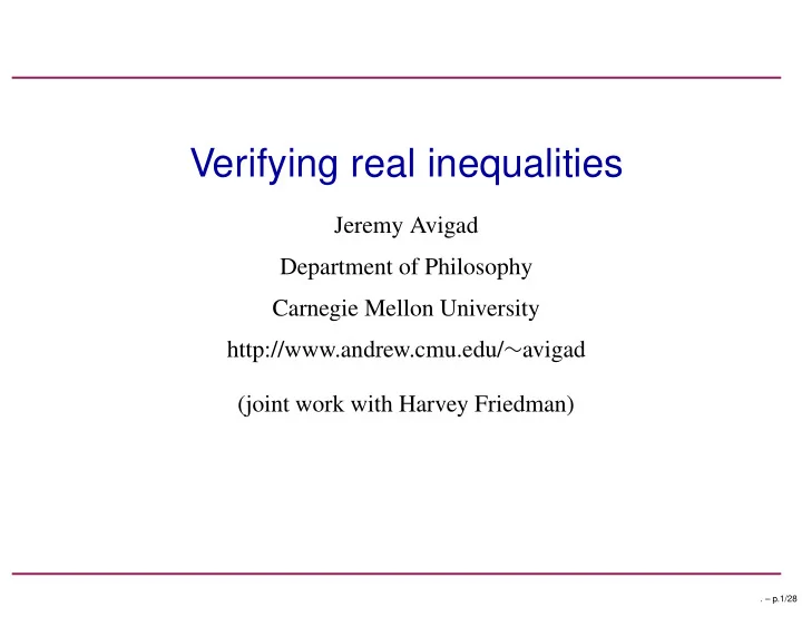
Verifying real inequalities Jeremy Avigad Department of Philosophy - - PowerPoint PPT Presentation

Verifying real inequalities

Jeremy Avigad Department of Philosophy Carnegie Mellon University http://www.andrew.cmu.edu/∼avigad (joint work with Harvey Friedman)

. – p.1/28

A characterization of mathematics

For centuries, mathematics was viewed as the science of quantity:

• Geometry = study of magnitude (continuous quantities)
• Arithmetic = study of number (discrete quantities)

Comparisons between quantities are central to the subject. We need better automated support for ordinary mathematical reasoning involving inequalities.

. – p.2/28

First example

Ramsey’s theorem tells us that for every k there is an N large enough, so that no matter how one colors the edges of the complete graph on N vertices red and blue, there is a homogeneous subset of size k. Here is a lower bound on N: Theorem (Erdös) For all k ≥ 2, if N < 2k/2, there is a coloring of the complete graph on N vertices with no homogeneous subset of size k. For k = 2 and k = 3 is it easy to check this by hand. For k ≥ 4, show that with nonzero probability, a random coloring has this property.

. – p.3/28

First example

For k ≥ 4, suppose N < 2k/2, and suppose we color each edge red with probability 1/2. The probability that any given subset of size k is homogeneous is 2−(k

2)+1.

So the probability of a homogeneous subset is at most N

k

• 2−(k

2)+1.

But N

k

• = N(N−1)(N−2)···(N−k+1)

k(k−1)···1

≤

Nk 2k−1.

So we have N k

• 2−(k

2)+1 ≤ N k

2k−1 2−(k

2)+1 < 2 k2 2 −(k 2)−k+2 = 2− k 2+2 ≤ 1.

. – p.4/28

Second example

• Proposition. When 0 ≤ x ≤ 1/2, we have x − x2 ≤ ln(1 + x) ≤ x.

Let’s do this without using the Maclaurin series! Suppose 0 ≤ x ≤ 1/2. From ex = 1 + x + x2/2 + . . ., we have ex ≥ 1 + x and hence ex2 ≥ 1 + x2. On the other hand, ex ≤ 1 + x + x2/2 + x2/4 + x2/8 + . . . = 1 + x + x2. So we have ex−x2 = ex/ex2 ≤ (1 + x + x2)/(1 + x2) ≤ 1 + x, by multiplying through. Taking logarithms, we have x − x2 ≤ ln(1 + x) ≤ x.

. – p.5/28

Third example

Here’s an inequality that comes up in Shapiro’s presentation of the Selberg proof of the prime number theorem. Assuming n ≤ (K/2)x 0 < C 0 < ε < 1 we have (1 + ε 3(C + 3)) · n < K x

. – p.6/28

Reflection

Here’s what these examples have in common:

• They are “typical.”
• They are straightforward.
• They are quantifier-free.
• They rely on basic arithmetic inferences.
• Verifying them formally is (currently) a pain in the neck.

(Mild uses of quantifiers come in with phrases like “sufficiently large,” or “choose N >> x.”) The challenge: figure out how to capture these automatically.

. – p.7/28

Real closed fields

Consider the first-order theory of R, 0, 1, +, ×, <. Theorem (Tarski). T has elimination of quantifiers, that is, every sentence in the language is provably equivalent to one that is quantifier-free. Hence T is decidable. Chronology:

• Alfred Tarski proved this around 1930 (finally published in 1948),

based on Sturm’s theorem.

• Abraham Robinson gave an easy model-theoretic proof in 1956,

based on Artin-Schreier.

• George Collins gave a practical method in 1975.
• Sean McLaughlin and John Harrison have recently implemented a

proof-producing version.

. – p.8/28

Real closed fields

But the story doesn’t end here.

• RCF procedures are slow (and arguably misguided, for the types of

inferences we are interested in).

• Worse: they do not extend to straightforward inferences with

monotone functions, trigonometric functions, exponentiation and logarithm, etc. Problem: nontrivial parts of mathematics are undecidable. Two options:

• Use full decision procedures in more restricted settings.
• Use “heuristic procedures” in more general settings.

Is there a middle ground? Let’s consider some strategies.

. – p.9/28

Idea 1: work backwards

Work backwards, using, for example, 0 < s, 0 < t ⇒ 0 < st and 0 < s < t ⇒ 1/t < 1/s. But backchaining is nondeterministic. For example:

• We also have s < 0, t < 0 ⇒ 0 < st and s < t < 0 ⇒ 1/t < 1/s.
• We can prove s + t + u < r + v by proving s + u < r and t ≤ v.
• We can also prove s + t + u < r + v by proving s + u < r + 3 and

t ≤ v − 3 or by proving s < (r + v)/2 and t + u < (r + v)/2.

. – p.10/28

Idea 2: work forwards

For example, from n ≤ (K/2)x, 0 < C, and 0 < ε < 1, we have

• C + 3 > 1
• 3(C + 3) > 1
• ε

3(C+3) < 1

• 1 +

ε 3(C+3) < 2

and hence (1 + ε 3(C + 3)) · n < 2(K/2)x = K x. But clearly we need some guidance!

. – p.11/28

Idea 3: combine local procedures

• Theorem. Suppose T1 and T2 are “locally finite” and decidable. Suppose

that the languages are disjoint, except for the equality symbol. Then the universal fragment of T1 ∪ T2 is decidable. In particular, if T1 and T2 have only infinite models, they are locally finite. This allows you to design decision procedures for individual theories and then put them together. With additional hypotheses on the source theories, the decision procedures can be made efficient (Nelson-Oppen, Shostak, ...).

. – p.12/28

Idea 3: combine local procedures

• Theorem. The theory of R, 0, +, < has quantifier-elimination, and so

is decidable. For universal formulas, Fourier-Motzkin is doubly exponential in principle, but works well in practice. More efficient methods are available (e.g. Weispfenning’s “test point” method).

• Theorem. The theory of R, 1, ·, < has quantifier-elimination and so is

decidable. In fact, modulo case splits on the signs of terms, this reduces to the previous theorem.

• Corollary. The universal fragment of the union of these two theories is

decidable.

. – p.13/28

Idea 3: combine local procedures

The bad news: the union of the two theories just described doesn’t include distributivity. The good news: many inferences don’t need it, except for constants (for example, 3(r + s) = 3r + 3s). The bad news: adding symbols for constants, or multiplication by constants, introduces nontrivial overlap between the languages. Nelson-Oppen methods break down. General question: what happens when you combine local procedures, when the theories have nontrivial overlap?

. – p.14/28

A theory for real inequalities

Specifically: let fa(x) = ax for rational constants a. Let Tadd[Q] be the theory of R, 0, 1, +, −, <, . . ., fa, . . .. Let Tmult[Q] be the theory of R, 0, 1, ×, ÷, n √·, <, . . . , fa, . . .. Let Tcommon[Q] = Tadd[Q] ∩ Tmult[Q]. Let T [Q] = Tadd[Q] ∪ Tmult[Q]. This theory seems to be very useful. Tadd[Q], Tmult[Q], Tcommon[Q] all have quantifier elimination. But the presence of the new symbols in the common language makes the situation much more complex.

. – p.15/28

A theory for real inequalities

Think of T [Q] as:

• real-closed fields without distributivity (except for constants)
• a shotgun wedding of the additive and multiplicative theories.

It seems to cover very many “obvious” calculations.

• Theorem. Let f (x1, . . . , xk) be a polynomial over Q. Then f is nonzero
• n [0, 1]k if and only if T [Q] proves that fact.

This provides a lower bound on the strength of T [Q] on universal

• assertions. For an upper bound:
• Theorem. T [Q] proves ∀x (x2 − 2x + 1 ≥ ε) if and only if ε < 0.

In fact, the size of a minimal interpolant depends on ε.

. – p.16/28

A theory for real inequalities

Here are some of our results.

• T [Q] has good normal forms.
• Valid equations are independent of the ordering.
• T [Q] is undecidable.
• In fact, the ∀∀∀∃ . . . ∃ fragment is complete r.e.
• Assuming that the solvability of Diophantine equations in the

rationals is undecidable, then so is the existential fragment of T [Q]. Most important:

• The universal fragment of T [Q] is decidable.

More generally, we consider theories T [F], for arbitrary computable subfields F of R.

. – p.17/28

Decidability of the universal fragment

Let ∀ x ϕ( x) be a universal formula of T [F]. By introducing variables to name subterms, we can reprexpress this as ϕ ≡ ∀ x (ϕadd( x) ∨ ϕmult( x)) where ϕadd and ϕmult are in the languages of Tadd[F], Tmult[F], respectively.

• Theorem. T [F] proves ∀

x ϕ iff there is a quantifier-free “interpolant” θ( x) in the language of Tcommon[F] such that

• Tadd[F] ∪ {¬ϕadd(

x)} ⊢ θ( x)

• Tmult[F] ∪ {¬ϕmult(

x)} ⊢ ¬θ( x).

. – p.18/28

Decidability of the universal fragment

In the Nelson-Oppen setting, there are only finitely many possible interpolants. The language of Tcommon[F] has atomic formulas xi ≤ ax j, xi < ax j. (We can assume each xi > 0, and x1 = 1.) Difficulties:

• There are infinitely many constants.
• There is no a priori bound on the size of the interpolant.
• Constants come from the subfield, F.

Nonetheless, with work, one can develop an algorithm to determine whether there is such an interpolant.

. – p.19/28

Decidability of the universal fragment

• Theorem. The following are equivalent:
• 1. T [F] doesn’t prove ϕ.
• 2. The union of Tadd[F] ∪ {¬ϕadd(

x)} and Tmult[F] ∪ {¬ϕmult( x)} is consistent.

• 3. There is a complete type Ŵ(

x) in Tcommon[F] such that

• Tadd[F] ∪ {¬ϕadd(

x)} ∪ Ŵ( x) and

• Tmult[F] ∪ {¬ϕmult(

x)} ∪ Ŵ( x) are both consistent. T [F] ⊢ ϕ iff for every complete type Ŵ( x) in the language of Tcommon[F], there is a finite subset Ŵ′( x) such that either ∀ x (

• Ŵ′(

x) → ϕadd( x))

• r

∀ x (

• Ŵ′(

x) → ϕmult( x)) holds in the reals.

. – p.20/28

Decidability of the universal fragment

One can characterize all the complete types, Ŵ( x), in terms of what they say about pairs {xi, x j}. With work, the assertion above can be expressed by a restricted class of formulas in the language of real closed fields, with a predicate for F. With more work, one can show that this class is decidable (assuming F is computable and F ∩ A is decidable).

. – p.21/28

Undecidability

• Theorem. There is a model of T [F] where the solutions to the equation

x(1 + x) = x + x2 are exactly the x ∈ F.

• Corollary. An existential sentence ϕ over F if and only if in any model
• f T [F], ϕ has witnesses among the a with a(1 + a) = a + a2.
• Corollary. If Diophantine equations in the rationals are unsolvable, then

so is the set of existential consequences of T [Q].

. – p.22/28

Undecidability

• Theorem. There is a model of T [F] and elements µ, κ, λ such that

solutions x ∈ [1, µ] to (κ + x)(λ + x) = κλ + κx + λx + x2 are exactly the positive integers.

• Corollary. Let ϕ be a Diophantine equation over the positive integers.

Then ϕ has a solution in the positive integers if and only for every model M of T [F], and every µ, κ, λ ∈ M, if {x ∈ [1, µ] | (κ + x)(λ + x) = κλ + κx + λx + x2} contains 1 and is closed under +1, then ϕ has solutions in that set.

• Corollary. The set of ∀∀∀∃ . . . ∃ consequence of T [F] is complete r.e.

. – p.23/28

Normal forms

One can simultaneously define normal forms and an ordering on terms in normal form. 4(1 + 3x1 + 4x1x7)2(x2

1x3 2 + 4x2 3x2 9)3

Two terms are provably equal if and only if they have the same normal form. In that case, they are provably equal in the theory without the ordering.

. – p.24/28

Heuristic procedures

Our decidability results are not practical. But the proofs provide ideas and guidelines. We propose the following strategy: given a sequent r1 < s1,r2 ≤ s2, . . . , rk < sk ⇒ t < u, put all terms in normal form, and try to refute r1 < s1,r2 ≤ s2, . . . ,rk < sk, u ≤ t. To do this, you need to find an interpolant. Iteratively use the additive and multiplicative parts to derive new inequalities, p < aq or p ≤ aq, between “subterms.”

. – p.25/28

Heuristic procedures

Disadvantages:

• The procedure is not complete (need disjunctions).
• The procedure may not terminate.
• Need to consider arbitrary pairs of subterms.

Advantages:

• The method has the right flavor: forward reasoning, but focusing on

“potentially useful” comparisons.

• It includes arithmetic and multiplicative decision procedures.
• It works on the kinds of examples I described above.

We expect that the method will work well in practice, but experimentation is needed.

. – p.26/28

Heuristic procedures

The method is, furthermore, open-ended and extensible:

• One can judiciously incorporate distributivity.
• One can judiciously incorporate disjunctions (case splits).
• One can add rules for ex, ln x, sin, cos, ...
• One can add general rules for monotone functions.

There are:

• interesting implementation issues
• interesting theoretical issues

. – p.27/28

Conclusions

Formally verified mathematics is becoming increasingly important:

• Proofs are getting very complex.
• Proofs rely on extensive computations.

New approaches are needed:

• Interesting fragments of mathematics are undecidable.
• Heuristic procedures are brittle, hard to extend, and unpredictable.

What we need are principled search procedures:

• Build heuristics on sound theory.
• Pay attention to data, and develop more useful classifications of

mathematical contexts. The work holds many engineering and theoretical challenges.

. – p.28/28