Vector Visualiza0on Applica0ons Climate Modeling Computational - PowerPoint PPT Presentation

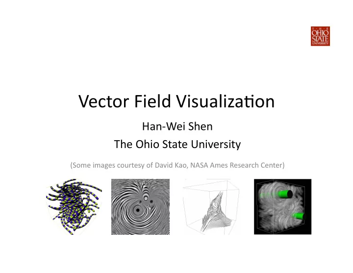
Vector Field Visualiza0on Han-Wei Shen The Ohio State University (Some images courtesy of David Kao, NASA Ames Research Center)

Vector Visualiza0on Applica0ons Climate Modeling Computational Fluid Dynamics Medical Applications Astronomy

Vector Field Visualiza0on • Vector field: F( u ) = v u : posi0on in the domain (x,y) in 2D (x,y,z) in 3D v : the vector (u,v) or (u,v,w) at u

Vector Field Visualiza0on • Vector field: F( u ) = v u : posi0on in the domain (x,y) in 2D (x,y,z) in 3D v : the vector (u,v) or (u,v,w) at u • Vectors are oPen defined at discrete points as aQributes at different 0me steps …

Methods for Experimental Flow Visualiza0on - Adding Foreign Material • Streaklines: dye injected from a fixed posi0on. By injec0ng the dye for a period of 0me, a line of dye in the fluid is visible • Timelines: a row of small par0cles (hydrogen bubbles) released at right angles to flow. The mo0on of the par0cles shows the fluid behavior • Pathlines: small par0cles (magnesium powder in liquid; oil drops in gas) are added to the fluid. Velocity is measured by photographing the mo0on of the par0cles with a known exposure 0me

Experimental Flow Visualization

Numerical Flow Visualiza0on Though numerical flow visualiza0on is not able to totally replicate the results from experimental flow visualiza0on, it has been widely accepted as an effec0ve mean to obtain accurate representa0on of the CFD flow solu0ons.

Numerical Flow Visualization – Basic Methods

Numerical Flow Visualization – Basic Methods Velocity Magnitude Contours Vector Arrow Plots Par0cle Traces - Streamlines

Visualiza0on Techniques I • Geometry-based methods: Render primi0ves from par0cle trajectories • 1D: streamlines, pathlines, streaklines • Line varia0ons: tubes, ribbons • 2D: stream surfaces • 3D: flow volumes

Visualiza0on Techniques II • Texture-based methods: Create texture paQerns following flow direc0ons – Line Integral Convolu0on – Texture Splates

Visualiza0on Techniques III • Topological-based methods: Extract features based on flow topology – Critical points – Vortex cores – Skin-friction lines

Par0cle Tracing Visualizing the flow direc0ons by releasing par0cles and calcula0ng a series of par0cle posi0ons based on the vector field

Par0cle Tracing Challenges • Displaying streamlines is a local technique because you can only visualize the flow direc0ons ini0ated from one or a few par0cles • When the number of streamlines is increased, the scene becomes cluQered • You need to know where to drop the par0cle seeds • Streamline computa0on is not cheap • It is much more difficult to predict the data access paQern

Seed Placement Density and distribu0on

Vector Glyphs • Display the en0re flow field in a single picture • Minimal user interven0on • Example: Hedgehogs (global arrow plots)

Example of hedgehogs

Varia0ons of hedgehogs

Line Integral Convolu0on (LIC)

Flow Line Computa0on

Flow Line Visualiza0on • One of the most fundamental flow visualiza0on techniques • Type of flow lines: – Streamline: a field line tangent to the velocity field at an instant in 0me – Pathline: the trajectory of a mass less par0cle released from a seed point over a period of 0me – Streakline: a line joining the posi0ons, at an instant in 0me, of par0cles released from a seed point – Timeline: a line connec0ng a row of par0le that are released simultaneously In a steady flow filed, streamlines, pathlines, and streaklines are iden0cal

Streamlines • Streamline: a line that is tangen0al to the instantaneous velocity direc0on (velocity is a vector, and it has a magnitude and a direc0on) • Release a par0cle into the flow and perform numerical integra/on t o compute the path of the par0cle

Pathlines • A pathline shows the trajectory of a single particle released from a fixed location (seed point) • Experimental method: marking a fluid par0cle and taking a 0me exposure photo of its mo0on will generate a pathline • This is similar to what you see when you take a long- exposure photograph of car lights on a freeway at night

Streaklines • S treakline : a line joining the posi0ons, at an instant in 0me, of all par0cles that were previously released from a fixed loca0on (seed point) • Con0nuously inject par0cles into the flow at each 0me step and track the paths of the par0cles • In a steady flow field, streamlines, pathlines, and streaklines are iden0cal. However, they can be very different in unsteady flows

Timelines • Timeline : a line connec0ng a row of par0cles that released simultaneously • Timelines are generated by injec0ng rows of par0cles at some fixed 0me interval

[Lane ‘96] e

Compu0ng Flow Lines by Par0cle Tracing • The path of a massless par0cle at posi0on p at 0me t can be described by the following ordinary differen0al equa0on: The image part with relationship ID rId3 was not found in the file. The image part with relationship ID rId5 was not found in the file. or steady flow unsteady flow

Compu0ng Flow Lines - Par0cle Tracing • The path of a massless par0cle at posi0on p at 0me t can be described by the following ordinary differen0al equa0on: The image part with relationship ID rId3 was not found in the file. The image part with relationship ID rId5 was not found in the file. or steady flow unsteady flow • And the posi0ons of the par0cle can be computed by Solved by numerical integra0on

Compu0ng Flow Lines - Par0cle Tracing • The path of a massless par0cle at posi0on p at 0me t can be described by the following ordinary differen0al equa0on: The image part with relationship ID rId3 was not found in the file. The image part with relationship ID rId5 was not found in the file. or steady flow unsteady flow • And the posi0ons of the par0cle can be computed by Solved by numerical integra0on

Numerical Integra0on • Discrete approxima0on of the con0nuous integra0on result v v(t) t

Numerical Integra0on • Discrete approxima0on of the con0nuous integra0on result v v(t) • Calculate area under curve for curve y(t) t – Trapezoidal approxima0on v v(t) t

Numerical Integra0on • Discrete approxima0on of the con0nuous integra0on result v v(t) • Calculate area under curve for curve y(t) t – Trapezoidal approxima0on v v(t) • Error related to the step size used • Below we describe a few popular methods of t numerical integra0on for par0cle tracing

Euler’s Method • Simple but lower accuracy Approxima0on p k+1 = p k + v ( p k ) x Δ t Ground True

Euler’s Method • Simple but lower accuracy Approxima0on p k+1 = p k + v ( p k ) x δ t Ground True • The equa0on can be derived from Taylor series expansion where y is one component of the P posi0on, and y’ is the one component of the velocity, h is the step size (Δ t ) Error

2 nd Order Runge-KuQa (RK2) • Improved accuracy, more commonly used p * = p k + v ( p k ) x δ t

2 nd Order Runge-KuQa (RK2) • Improved accuracy, more commonly used p * = p k + v ( p k ) x δ t p k+1 = p k + ( v ( p k ) + v ( p * ) ) x δ t/2 • Can also be derived from Taylor’s series (next slide)

2 nd Order Runge-KuQa (RK2) • Improved accuracy from Euler for ODE • Differen0a0ng the above equa0on • From Taylor series expansion: V(P k ) V(P * )

4 th Order Runge-KuQa (RK4) • BeQer accuracy, recommended a = 2 δ t v ( p k ), b = 2 δ t v ( p k + a /2), c = 2 δ t v ( p k + b /2) d = 2 δ t v ( p k + c /2), p k+1 = p k + ( a +2 b +2 c + d )/6

Put it All Together Par0cle Tracing Algorithm 1. Specify a seed posi0on p(0), t = 0 2. Perform cell search to locate the cell that contains the p(t) 3. Interpolate the velocity field to determine the velocity at p(t) 4. Advance the par0cle from p(t) to p(t+Δ t ) using a numerical integra0on method 5. Repeat from step 2 un0l the par0cle moves a certain distance or goes out of bound

Line Integral Convolu0on

Line Integral Convolution

Motivation • To visualize steady 2D vector fields, or flows near the body of the model (surface flows) • To create images similar to experimental oil-flow visualization • To overcome the drawback of traditional flow visualization techniques

Streamline Problems • Seed placement is non trivial • Trial and error • Need prior knowledge • Unsatisfactory visualization • Grid spacing may vary • Difficult to control streamline lengths • Discontinued flow lines

Streamlines Uneven streamline density and lengths

Streamline and LIC Comparison Streamlines LIC

LIC – Cabral & Leedom ‘93

Line Integral Convolution • From each pixel, streamlines are computed in both directions

Line Integral Convolution • From each pixel, streamlines are computed in both directions

Line Integral Convolution • From each pixel, streamlines are computed in both directions • Pixel values from the input noise image are summed together with weights

Line Integral Convolution • From each pixel, streamlines are computed in both directions • Pixel values from the input noise image are summed together with weights