Unweighted directed graphs Announcements Midterm & gradescope - PowerPoint PPT Presentation
Unweighted directed graphs Announcements Midterm & gradescope - will get an email today to register (username name is your email) - tests should appear by next Monday (nothing there now) Graph A directed graph G is a set of edges and
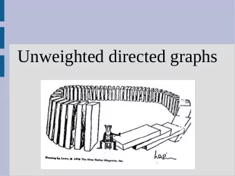
Unweighted directed graphs
Announcements Midterm & gradescope - will get an email today to register (username name is your email) - tests should appear by next Monday (nothing there now)
Graph A directed graph G is a set of edges and vertices: G = (V, E) Two common ways to represent a graph: a b -Adjacency matrix -Adjacency list c d
Graph An adjacency matrix has a 1 in row i and column j if you can go from node i to node j
Graph An adjacency list just makes lists out of each row (list of edges out from every vertex)
Graph Difference between adjacency matrix and adjacency list?
Graph Difference between adjacency matrix and adjacency list? Matrix is more memory O(|V| 2 ), less computation: O(1) lookup List is less memory O(E+V) if sparse, more computation: O(branch factor)
Graph Adjacency matrix, A=A 1 , represents the number of paths from row node to column node in 1 step Prove: A n is the number of paths from row node to column node in n steps
Graph Proof: Induction Base: A 0 = I, 0 steps from i is i Induction: (Assume A n , show A n+1 ) Let a n i,j = i th row, j th column of A n Then a n+1 i,j = ∑ k a n i,k a 1 k,j This is just matrix multiplication
Breadth First Search Overview Create first-in-first-out (FIFO) queue to explore unvisited nodes https://www.youtube.com/watch?v=nI0dT288VLs
Breadth First Search Overview Consider the graph below Suppose we wanted to get from “a” to “c” using breadth first search
BFS Overview To keep track of which nodes we have seen, we will do: White nodes = never seen before Grey nodes = nodes in Q Black nodes = nodes that are done To keep track of who first saw nodes I will make red arrows (π in book)
BFS Overview First, we add the start to the queue, so Q = {a} Then we will repeatedly take the left-most item in Q and add all of its neighbors (that we haven't seen yet) to the Q on the right
BFS Overview Q = {a} Left-most = a White neighbors = b & d New Q = {b, d}
BFS Overview Q = {b, d} Left-most = b White neighbors = e New Q = {d, e}
BFS Overview Q = {d, e} Left-most = d White neighbors = c & f & g New Q = {e, c, f, g}
BFS Overview Q = {e, c, f, g} Left-most = e White neighbors = (none) New Q = {c, f, g}
BFS Overview Q = {c, f, g} Left-most = c Done! We found c, backtrack on red arrows to get path from “a”
Depth First Search Overview Create first-in-last-out (FILO) queue to explore unvisited nodes
Depth First Search Overview You can solve mazes by putting your left-hand on the wall and following it (i.e. left turns at every intersection)
Depth First Search Overview You can solve mazes by putting your left-hand on the wall and following it (i.e. left turns at every intersection)
Depth First Search Overview This is actually just depth first search (add nodes to the “right” first) D E A F I G H C B J
Depth First Search Overview Q = {A} Right most = A White neighbors = {B} New Q = {B}
Depth First Search Overview Q = {B} Right most = B White neighbors = {C, D} New Q = {C, D}
Depth First Search Overview Q = {C, D} Right most = D White neighbors = {H, E} New Q = {C, H, E}
Depth First Search Overview Q = {C, H, E} Right most = E White neighbors = {F, G} New Q = {C, H, F, G}
Depth First Search Overview Q = {C, H, F, G} Right most = G White neighbors = {} New Q = {C, H, F}
Depth First Search Overview Q = {C, H, F} Right most = F White neighbors = {} New Q = {C, H}
Depth First Search Overview Q = {C, H} Right most = H White neighbors = {I, J} New Q = {C, I, J}
Depth First Search Overview Q = {C, I, J} Right most = J J is exit, we are done
BFS and DFS in trees Solve problems by making a tree of the state space max min max
BFS and DFS in trees Often times, fully exploring the state space is too costly (takes forever) Chess: 10 47 states (tree about 10 123 ) Go: 10 171 states (tree about 10 360 ) At 1 million states per second... Chess: 10 109 years (past heat death Go: 10 346 years of universe)
BFS and DFS in trees BFS prioritizes “exploring” DFS prioritizes “exploiting” White to move Black to move
BFS and DFS in trees BFS benefits? DFS benefits?
BFS and DFS in trees BFS benefits? -if stopped before full search, can evaluate best found DFS benefits? -uses less memory on complete search
BFS and DFS in graphs BFS: shortest path from origin to any node DFS: find graph structure Both running time of O(V+E)
Breadth first search BFS(G,s) // to find shortest path from s for all v in V v.color=white, v.d=∞,v.π=NIL s.color=grey, v.d=0 Enqueue(Q,s) while(Q not empty) u = Dequeue(Q,s) for v in G.adj[u] if v.color == white v.color=grey, v.d=u.d+1, v.π=u Enqueue(Q,v) u.color=black
Breadth first search Let δ(s,v) be the shortest path from s to v After running BFS you can find this path as: v.π to (v.π).π to ... s (pseudo code on p. 601, recursion)
BFS correctness Proof: contradiction Assume δ(s,v) ≠ v.d v.d > δ(s,v) (Lemma 22.2, induction) Thus v.d > δ(s,v) Let u be previous node on δ(s,v) Thus δ(s,v) = δ(s,u)+1 and δ(s,u) = u.d Then v.d > δ(s,v) = δ(s,u)+1 = u.d+1
BFS correctness v.d > δ(s,v) = δ(s,u)+1 = u.d+1 Cases on color of v when u dequeue, all cases invalidate top equation Case white: alg sets v.d = u.d + 1 Case black: already removed thus v.d < u.d (corollary 22.4) Case grey: exists w that dequeued v, v.d = w.d+1 < u.d+1 (corollary 22.4)
Depth first search DFS(G) for all v in V v.color=white, v.π=NIL time=0 for each v in V if v.color==white DFS-Visit(G,v)
Depth first search DFS-Visit(G,u) time=time+1 u.d=time, u.color=grey for each v in G.adj[u] if v.color == white v.π=u DFS-Visit(G,v) u.color=black, time=time+1, u.f=time
Depth first search Edge markers: Consider edge u to v C = Edge to black node (u.d > v.f) B = Edge to grey node (u.f < v.f) F = Edge to black node (u.f > v.f)
Depth first search DFS can do topographical sort Run DFS, sort in decreasing finish time
Weighted graphs
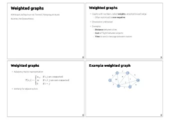
Weighted graph Edges in weighted graph are assigned a weight: w(v 1 , v 2 ), v 1 , v 2 in V If path p = <v 0 , v 1 , ... v k > then the weight is: w(p) = ∑ k i=0 (v i-1 ,v i ) Shortest Path: δ(u,v): min{w(p) : v 0 =u,v k =v)}
Shortest paths Today we will look at single-source shorted paths This finds the shortest path from some starting vertex, s, to any other vertex on the graph (if it exists) This creates G π , the shortest path tree
Shortest paths Optimal substructure: Let δ(v 0 ,v k )=p, then for all 0 < i < j < k, δ(v i ,v j )=p i,j = <v i , v i+1 , ... v j > Proof? Where have we seen this before?
Shortest paths Optimal substructure: Let δ(v 0 ,v k )=p, then for all 0 < i < j < k, δ(v i ,v j )=p i,j = <v i , v i+1 , ... v j > Proof? Contradiction! Suppose w(p' i,j ) < p( i,j ), then let p' 0,k = p 0,i p' i,j p j,k then w(p' 0,k ) < w(p)
Relaxation We will only do relaxation on the values v.d (min weight) for vertex v Relax(u,v,w) if(v.d > u.d + w(u,v)) v.d = u.d+w(u,v) v.π=u
Relaxation We will assume all vertices start with v.d=∞,v.π=NIL except s, s.d=0 This will take O(|V|) time This will not effect the asymptotic runtime as it will be at least O(|V|) to find single-source shortest path
Relaxation Relaxation properties: 1. δ(s,v) < δ(s,u) + δ(u,v) (triangle inequality) 2. v.d > δ(s,v), v.d is monotonically decreasing 3. if no path, v.d =δ(s,v) =∞ 4. if δ(s,v), when (v.π).d=δ(s,v.π) then relax(v.π,v,w) causes v.d=δ(s,v) 5. if δ(v 0 ,v k ) = p 0,k , then when relaxed in order (v 0 , v 1 ), (v 1 , v 2 ), ... (v k-1 ,v k ) then v k.d =δ(v 0 ,v k ) even if other relax happen 6. when v.d=δ(s,v) for all v in V, G π is shortest path tree rooted at s
Directed Acyclic Graphs DFS can do topological sort (DAG) Run DFS, sort in decreasing finish time
Directed Acyclic Graphs DAG-shortest-paths(G,w,s) topologically sort G initialize graph from s for each u in V in topological order for each v in G.Adj[u] Relax(u,v,w) Runtime: O(|V| + |E|)
Depth first search
Directed Acyclic Graphs Correctness: Prove it!
Directed Acyclic Graphs Correctness: By definition of topological order, When relaxing vertex v, we have already relaxed any preceding vertices So by relaxation property 5, we have found the shortest path to all v
BFS (unweighted graphs) Create FIFO queue to explore unvisited nodes
Dijkstra Dijkstra's algorithm is the BFS equivalent for non-negative weight graphs
Dijkstra Dijkstra(G,w,s) initialize G from s Q = G.V, S = empty while Q not empty u = Extract-min(Q) S optional S = S U {u} for each v int G.Adj[u] relax(u,v,w)
Dijkstra
Dijkstra Runtime?
Recommend
More recommend
Explore More Topics
Stay informed with curated content and fresh updates.

