Unsupervised Data Discretization of Mixed Data Types Jee Vang - PDF document

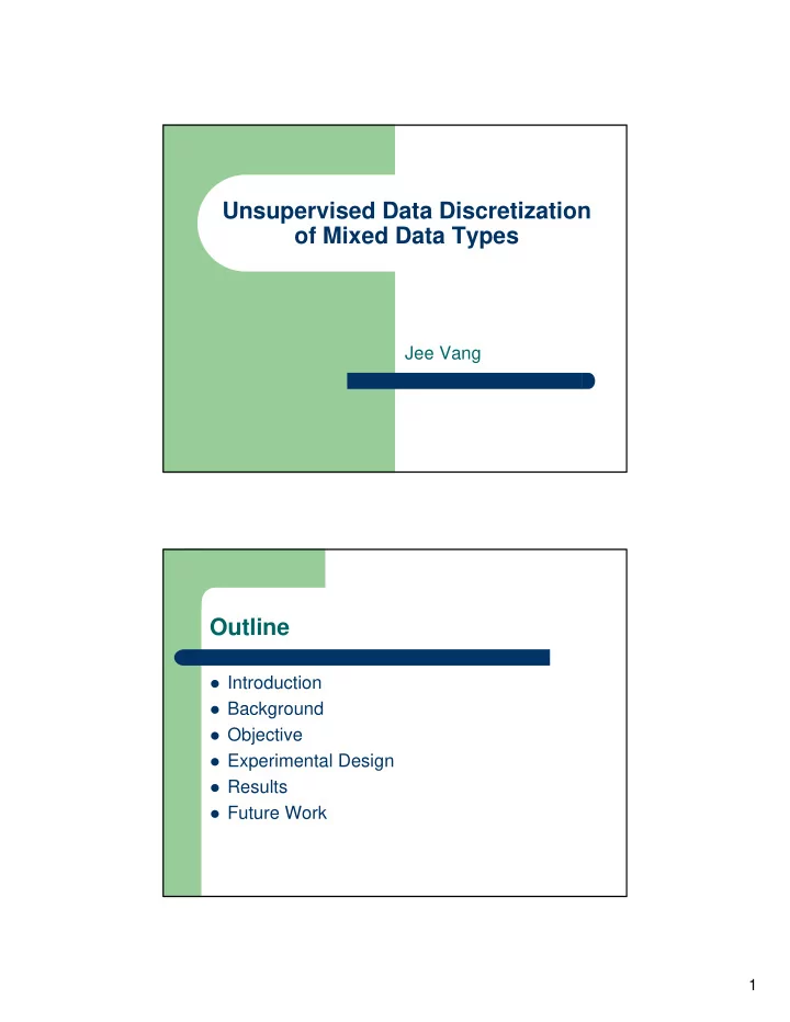
Unsupervised Data Discretization of Mixed Data Types Jee Vang Outline � Introduction � Background � Objective � Experimental Design � Results � Future Work 1

Introduction � Many algorithms in data mining, machine learning, and artificial intelligence operate only on either numeric or categorical data � Datasets often contain mixed types � Discretization is the process of transforming continuous variables to categorical variables – Few discretization algorithms address interdependence between variables in dataset with mixed type – Even fewer address such concerns in the absence of class label in the dataset Background - Discretization � Discretization – Static vs dynamic – Supervised vs unsupervised – Local vs global – Top-down vs bottom-up – Direct vs incremental � Only one known discretization algorithm that addresses dataset with mixed data types, is unsupervised, and considers variable interdependencies – Based on principal component analysis (PCA) and frequent itemset mining (FIM), PCA+FIM 2

Background – The Dataset � Dataset consists of 272 patients with drug abuse problems treated from November 1997 to March 2003; 60 patients removed due to inadequate follow- up; 3 patients removed due to unavailable demographics data; end up with 209 patients � A total of 13 variables were monitored – Binary: system type, technical violation, race, gender – Continuous: arrest, drug test, employment, homeless shelter, mental hospitalization, physical hospitalization, incarceration, treatment, age Objective � Quantitatively compare the preservation of correlation in the categorical domain after discretization in the continuous domain � Benchmark PCA+FIM with equal-width (EW) and equal-frequency (EF) approaches � Measuring how much correlation is preserved will be accomplished by using Spearman and Kendall correlation tests 3

Experimental Designs � Procedure – 1. measure the pair-wise correlations in the continuous domain – 2. input data set into discretization algorithms – 3. measure the pair-wise correlations in the categorical domain – 4. use Spearman or Kendall ranked-based correlation tests to observe much correlation is preserved between correlations in continuous (step 1) and categorical domain (step 2) Experimental Designs – Discretization Algorithms � PCA+FIM (Java, BLAS/LAPACK) 1. normalize and mean center data – 2. compute correlation matrix – 3. compute eigenvalues/eigenvectors of correlation matrix; keep – set of eigenvectors whose eigenvalues account for 95% of the variance 4. project data into eigenspace – 5. discretize variables in eigenspace by generating cutpoints – 6. project cutpoints back to original representation space – � EW (Data PreProcessor) K intervals of equal-widths are produced – � EF (Data PreProcessor) K intervals with equal frequency of data points are produced – 4

Experimental Designs – Pair-wise Correlation Measures � Continuous pair – Pearson – Kendall – Spearman � Categorical pair – Phi – Mutual information � Continuous-binomial pair – Point biserial Results - Cutpoints � Objective is not primarily to judge qualitatively (i.e. how meaningful are the cutpoints) � PCA+FIM and EF produce less cutpoints � EW produces more cutpoints 5

Results – Comparing Pearson correlation to phi and mutual information correlation Pearson - Phi Spearman Kendall PCA+FIM 0.15 0.09 EW 0.00 0.02 EF 0.13 0.07 Pearson – Mutual Information Spearman Kendall PCA+FIM 0.15 0.10 EW -0.10 -0.06 EF 0.11 0.08 Results – Comparing Spearman correlation to phi and mutual information correlation Spearman - Phi Spearman Kendall PCA+FIM 0.14 0.09 EW 0.46 0.33 EF 0.12 0.07 Spearman – Mutual Information Spearman Kendall PCA+FIM 0.15 0.11 EW 0.22 0.16 EF 0.09 0.07 6

Results – Comparing Kendall correlation to phi and mutual information correlation Kendall - Phi Spearman Kendall PCA+FIM 0.16 0.10 EW -0.25 -0.17 EF -0.01 -0.01 Kendall – Mutual Information Spearman Kendall PCA+FIM 0.19 0.14 EW -0.35 -0.20 EF 0.03 0.01 Results – Interpretation of correlation preservation � If Pearson correlation is used to measure correlation in the continuous domain, PCA+FIM will produce a discretized dataset preserving the most correlation � If Spearman correlation is used to measure correlation in the continuous domain, EW will produce a discretized dataset preserving the most correlation � EF seems to preserve the least correlations in the categorical domain from the continuous domain � PCA+FIM shows consistency in correlation preservation 7

Future Work � Implement k-nearest neighbor approach in PCA+FIM discretization algorithm � Test on other datasets References � Anderson, E., Bai, Z., Bischof, C., Blackford, S., Demmel, J., Dongarra, J., Du Croz, J., Greenbaum, A., Hammarling, S., McKenney, A., and Sorensen, D. LAPACK Users' Guide. Society for Industrial and Applied Mathematics, Philadelphia, PA: 1999. � Cheng, J. “Data PreProcessor.” http://www.cs.ualberta.ca/~jcheng/prep.htm, 7 May 2006. � Mehta, S., Parthasarathy , S., and Yang, H., “Toward Unsupervised Correlation Preserving Discretization,” IEEE Transactions on Knowledge and Data Engineering, vol. 17, no. 9, pp. 1174-1185, Sept., 2005. 8