Universality for the dimer model Nathana el Berestycki University - PowerPoint PPT Presentation

Universality for the dimer model Nathana¨ el Berestycki University of Cambridge with Benoit Laslier (Paris) and Gourab Ray (Cambridge) Les Diablerets, February 2017

The dimer model Definition G = bipartite finite graph, planar Dimer configuration = perfect matching on G : each vertex incident to one edge Dimer model: uniformly chosen configuration On square lattice, equivalent to domino tiling.

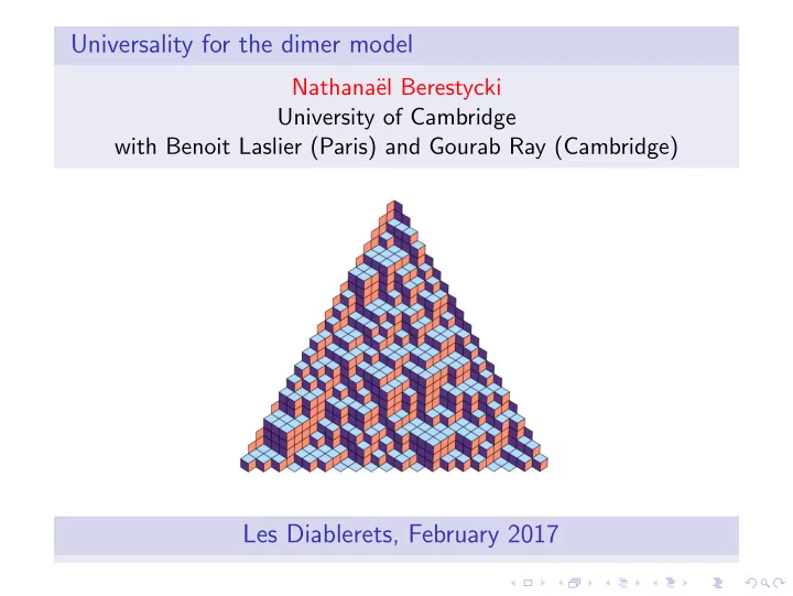
Dimer model as a random surface Can describe the dimer model through a height function. Hence view as random surface. Example: honeycomb lattice Dimer = lozenge tiling Equivalently: stack of 3d cubes.

Large scale behaviour? Main Question: What is large scale behaviour of height function?

Background Classical model of statistical mechanics: Kasteleyn, Temperley–Fisher 1960s Kenyon, Propp, Okounkov, Sheffield, Dub´ edat,... 1990s+ “Exactly Solvable”: determinantal structure m n m + 1) + 2 i cos( π k π j � 1 / 2 � � � � e.g., Z m , n = � 2 cos( n + 1) j =1 k =1 Analysis via: discrete complex analysis, Schur polynomials, Young tableaux, algebraic geometry... + Connection to SLE Mapping to other models: Tilings, 6-vertex, XOR Ising, Uniform Spanning Trees (UST)

Arctic circle phenomenon Some regions can be frozen, other liquid (temperate) Depends on boundary conditions in sensitive way Interface between frozen / liquid = arctic circle

Algebraic curves Cardioid: Aztec diamond: Kenyon–Okounkov–Sheffield Jockusch, Propp and Shor 1996 2006

Main questions (bis) Fluctuations Is there universality? (in the temperate region) Is there conformally invariance?

Main theorem Let h # δ = height function on hexagonal lattice, mesh-size = δ. Theorem (B.–Laslier–Ray 2016) Assume D is Jordan domain and boundary conditions of height lie in plane P ⊂ R 3 . h # δ − E ( h # δ ) 1 ◦ ℓ − − − → χ h GFF , δ δ → 0 where ℓ = linear map h GFF = Gaussian free field with Dirichlet boundary conditions. √ χ = 1 / 2. (Convergence in distribution in H − 1 − ε .)

What is the Gaussian free field? Informally, P ( f ) = 1 � − 1 � � |∇ f | 2 Z exp df 2 D GFF = canonical random function on D . But too rough to be a function Rigorously: in Sobolev space H − s , ∀ s > 0 � � � ( h GFF , f ) ∼ N 0 , G D ( x , y ) f ( x ) f ( y ) dxdy D where G D ( · , · ) = − ∆ − 1 Green’s function in D .

Novelty of approach Universality of fluctuations Insight as to why GFF universal? Needed: SRW → BM on certain graph. Does not fundamentally rely on exact solvability Instead: imaginary geometry and SLE Robustness Recover Kenyon 2000 (flat case with smooth D ) Extends to Dimer Model on isoradial graphs (extends Li 2014) Dimer model in random environment Work in progress: compact Riemann surfaces with no boundary etc.

Temperley’s bijection Benoit explained: dimer configurations with given slope ⇐ ⇒ UST in associated T-graph. Dimer configurations ↔ UST on T-graph Height function ↔ Winding of branches in tree New goal: Study winding of branches in Uniform Spanning Trees. Question How much do you wind around in a random maze?

Winding in UST Question How much do you wind around in a random maze? Answer: the GFF ! Let h # δ = winding of branches in UST. Real main theorem Assume ( ⋆ ). 1 h # δ − E ( h # δ ) − − − → χ h GFF , δ → 0 h GFF = Gaussian free field (Dirichlet boundary conditions). √ χ = 1 / 2. Note: E ( h # δ ) itself is not universal, only fluctuations!

Assumptions for the theorem Holds under very general assumptions: (1) Simple Random Walk on G # δ converges to Brownian motion (2) Uniform crossing condition: (“Russo–Seymour–Welsh” estimate) (3) Bounded density of vertices; edges have bounded winding

Ideas for the proof: working in the continuum 0 − 11 0 11

Scaling limit of Uniform Spanning Tree Theorem (Lawler, Schramm, Werner ’03, Schramm ’00) D ⊂ C ◮ Uniform spanning tree on D ∩ δ Z 2 → “A continuum tree” (continuum uniform spanning tree). ◮ Branches of the continuum tree are SLE 2 curves. Yadin–Yehudayoff 2010: universality (assuming convergence of SRW to BM).

Relations between SLE and GFF Theorem (Schramm–Sheffield) “Level lines” of the GFF are given by SLE 4 curves.

Imaginary Geometry Miller–Sheffield: “flow lines of GFF /χ are SLE κ curves”, provided: √ κ 2 χ = √ κ − 2 . Meaning: there is a coupling ( h , η ) such that h = GFF , η = SLE κ , such that λ + arg f ′ t − λ + arg f ′ t In other words, the values of the GFF along the curve records “winding” of the SLE.

Flow lines of GFF: e ih /χ . χ = 31 . 97 ... , flow lines = SLE 1 / 256 (Miller–Sheffield).

Flow lines of GFF: e ih /χ . χ = 11 . 23 ... , flow lines = SLE 1 / 32 (Miller–Sheffield).

Flow lines of GFF: e ih /χ . χ = 7 . 88 ... , flow lines = SLE 1 / 16 (Miller–Sheffield).

Flow lines of GFF: e ih /χ . χ = 2 . 47 ... , flow lines = SLE 1 / 2 (Miller–Sheffield).

Flow lines of GFF: e ih /χ . √ χ = 2, flow lines = SLE 2 (Miller–Sheffield). Suggests winding of continuum UST is (1 /χ ) GFF.

Proof of convergence, 1/4 winding h # δ − − − − → UST ↓ ↓ ? winding − − − − → Continuum UST h GFF Step 1: Making sense of intrinsic winding of rough curves. Let γ : [0 , 1] → C smooth, simple curve. Let W ( γ, z ) = topological winding around z and let � 1 arg γ ′ ( s ) ds W int ( γ ) = intrinsic winding of γ = 0 = π 2 ( # left turns - # right turns in discrete) .

Proof of convergence, 1/4. Lemma W int ( γ ) = W ( γ, γ (0)) + W ( γ, γ (1)) . Let h t ( z ) = intrinsic winding of branch to z , truncated at capacity t , followed by segment connecting to z . Theorem (B.–Laslier–Ray) h t − E ( h t ) → 1 χ h GFF (almost surely in H − 1 − ε ). Relies on Miller–Sheffield, + deformation of intrinsic winding under conformal maps.

Proof of convergence, 2/4 z 3 z 4 z 5 z 2 z 1 Step 2: The blue parts are roughly independent. Multiscale coupling, based on Schramm’s finiteness theorem: Fix k ≥ 1. We show UST in small neighbourhoods of z 1 , . . . , z k can be coupled to independent full-planes UST (with good probability).

Proof of convergence, 3/4 Step 3: method of moments Overall, if coupling successful: h # δ ≈ h t + e t ≈ h GFF + e t e t − E ( e t ) ≈ independent from point to point with mean zero. Fix test function f , � � ( h # δ , f ) k = h # δ ( z 1 ) f ( z 1 ) . . . h # δ ( z k ) f ( z k ) dz 1 . . . dz k . . . Convergence of E ok if coupling successful.

Proof of convergence, 4/4 Step 4: a priori winding estimates When coupling fails, need a priori bounds on winding, eg: Lemma (Stretched exponential tails for winding of LERW) Fix t > − 10 log( | v − ∂ D | ) . Then | h # δ t 1 ( v ) − h # δ < Ce − cn α . � � sup t 2 ( v ) | > n P t ≤ t 1 , t 2 ≤ t +1 Uses only uniform crossing assumption (RSW). Then separate argument for tightness in H − 1 − ε .

Robustness Work in progress Compact Riemann surfaces with no boundary, eg torus. To infinity and beyond... On torus, height function → compactified GFF. This answers question by Dub´ edat–Gheissari Universal limit for Cycle-Rooted Spanning Forest (extends Kassel–Kenyon) A theory of Imaginary Geometry on Riemann surfaces

Robustness Future work: General boundary conditions; multiply connected case etc. Interacting dimers and space-filling SLE κ ′ . Pictures acknowledgements: Kenyon, Miller, Sheffield, Lee, Ray ...