Unit #2: Complexity Theory and Asymptotic Analysis CPSC 221: - PowerPoint PPT Presentation
Unit #2: Complexity Theory and Asymptotic Analysis CPSC 221: Algorithms and Data Structures Lars Kotthoff 1 larsko@cs.ubc.ca 1 With material from Will Evans, Steve Wolfman, Alan Hu, Ed Knorr, and Kim Voll. Asymptotic Behaviour image from
Unit #2: Complexity Theory and Asymptotic Analysis CPSC 221: Algorithms and Data Structures Lars Kotthoff 1 larsko@cs.ubc.ca 1 With material from Will Evans, Steve Wolfman, Alan Hu, Ed Knorr, and Kim Voll.
Asymptotic Behaviour image from Wikipedia
Asymptotic Behaviour ▷ We measure runtime as a function of the input size n . ▷ We don’t care about constants and constant factors. ▷ We are most interested what happens when n gets big.
Big-O Notation T ( n ) ∈ O ( f ( n )) if there are positive constants c and n 0 such that T ( n ) ≤ cf ( n ) for all n ≥ n 0 .
Asymptotic Notation ▷ T ( n ) ∈ O ( f ( n )) if there are positive constants c and n 0 such that T ( n ) ≤ cf ( n ) for all n ≥ n 0 . ▷ T ( n ) ∈ Ω( f ( n )) if there are positive constants c and n 0 such that T ( n ) ≥ cf ( n ) for all n ≥ n 0 . ▷ T ( n ) ∈ Θ( f ( n )) if T ( n ) ∈ O ( f ( n )) and T ( n ) ∈ Ω( f ( n )) . ▷ T ( n ) ∈ o ( f ( n )) if for any positive constant c , there exists n 0 such that T ( n ) < cf ( n ) for all n ≥ n 0 . ▷ T ( n ) ∈ ω ( f ( n )) if for any positive constant c , there exists n 0 such that T ( n ) > cf ( n ) for all n ≥ n 0 .
Examples 10 , 000 n 2 + 25 n ∈ Θ( n 2 ) 10 − 10 n 2 ∈ Θ( n 2 ) n log n ∈ O ( n 2 ) n log n ∈ Ω( n ) n 3 + 4 ∈ o ( n 4 ) n 3 + 4 ∈ ω ( n 2 )
Analyzing Code // Linear search find(key, array) for i = 0 to length(array) - 1 do if array[i] == key return i return -1 4) How does T ( n ) = 2 n + 1 behave asymptotically? What is the appropriate order notation? ( O , o , Θ , Ω , ω ?)
Asymptotically smaller? n 3 + 2 n 2 100 n 2 + 1000 versus 12000 n 3 + 2 n 2 10000 100 n 2 + 1000 8000 6000 4000 2000 0 1 2 3 4 5 6 7 8 9 10
Asymptotically smaller? n 3 + 2 n 2 100 n 2 + 1000 versus 9e+06 12000 n 3 + 2 n 2 n 3 + 2 n 2 8e+06 10000 100 n 2 + 1000 7e+06 100 n 2 + 1000 6e+06 8000 5e+06 6000 4e+06 3e+06 4000 2e+06 2000 1e+06 0 0 1 2 3 4 5 6 7 8 9 10 20 40 60 80 100120140160180200
Asymptotically smaller? n 0 . 1 versus log 2 n 3.5 3 n 0 . 1 2.5 log 2 n 2 1.5 1 0.5 0 1 2 3 4 5 6 7 8 9 10
Asymptotically smaller? n 0 . 1 versus log 2 n 3.5 70 3 60 n 0 . 1 2.5 n 0 . 1 50 log 2 n log 2 n 2 40 1.5 30 1 20 0.5 10 0 0 1 2 3 4 5 6 7 8 9 10 0 2e+17 4e+17 6e+17 8e+17 1e+18
Asymptotically smaller? n + 100 n 0 . 1 versus 2 n + 10 log 2 n 140 120 n + 100 n 0 . 1 100 2 n + 10 log 2 n 80 60 40 20 0 1 2 3 4 5 6 7 8 9 10
Asymptotically smaller? n + 100 n 0 . 1 versus 2 n + 10 log 2 n 2.5e+18 140 n + 100 n 0 . 1 120 2e+18 n + 100 n 0 . 1 2 n + 10 log 2 n 100 2 n + 10 log 2 n 1.5e+18 80 60 1e+18 40 5e+17 20 0 0 1 2 3 4 5 6 7 8 9 10 0 2e+17 4e+17 6e+17 8e+17 1e+18
Typical asymptotics Tractable ▷ constant: Θ(1) ▷ logarithmic: Θ(log n ) ( log b n , log n 2 ∈ Θ(log n ) ) ▷ poly-log: Θ( log k n ) ( log k n ≡ (log n ) k ) ▷ linear: Θ( n ) ▷ log-linear: Θ( n log n ) ▷ superlinear: Θ( n 1+ c ) ( c is a constant > 0 ) ▷ quadratic: Θ( n 2 ) ▷ cubic: Θ( n 3 ) ▷ polynomial: Θ( n k ) ( k is a constant) Intractable ▷ exponential: Θ( c n ) ( c is a constant > 1 )
Sample asymptotic relations ▷ { 1 , log n, n 0 . 9 , n, 100 n } ⊂ O ( n ) ▷ { n, n log n, n 2 , 2 n } ⊂ Ω( n ) ▷ { n, 100 n, n + log n } ⊂ Θ( n ) ▷ { 1 , log n, n 0 . 9 } ⊂ o ( n ) ▷ { n log n, n 2 , 2 n } ⊂ ω ( n )
Analyzing Code ▷ single operations: constant time ▷ consecutive operations: sum operation times ▷ conditionals: condition time plus max of branch times ▷ loops: sum of loop-body times ▷ function call: time for function Above all, use your head!
Runtime example #1 for i = 1 to n do for j = 1 to n do sum = sum + 1
Runtime example #2 i = 1 while i < n do for j = i to n do sum = sum + 1 i++
Recommend
More recommend
Explore More Topics
Stay informed with curated content and fresh updates.
