Understanding the Long-Term Self-Similarity of Internet Traffic - PowerPoint PPT Presentation
Understanding the Long-Term Self-Similarity of Internet Traffic Steve Uhlig and Olivier Bonaventure InfoNet group University of Namur, Belgium E-mail : suhlig,obonaventure @info.fundp.ac.be URL : http://www.infonet.fundp.ac.be/
✁ � ✂ Understanding the Long-Term Self-Similarity of Internet Traffic Steve Uhlig and Olivier Bonaventure InfoNet group University of Namur, Belgium E-mail : suhlig,obonaventure @info.fundp.ac.be URL : http://www.infonet.fundp.ac.be/ c QOFIS’2001 S. Uhlig (University of Namur, Belgium) Page 1
✌ ✡ � ✂ ✁ � � � ☛☞ ✆✝ ✟ ✞✟✠ The Traffic Trace Measurement study Collect Netflow records for a Belgian ISP during days. Netflow : total volume between and (for layer-4 flows) ✂☎✄ All the incoming traffic (interdomain). Studied ISP BELNET : research and government ISP ( http://www.belnet.be ) – high bandwidth links to two transit ISPs, E3 link to SURFNET/AMS-IX, OC-3 link to BNIX, 1.5 DS3 links to TEN-155 – Main user : University attached to E3 backbone c QOFIS’2001 S. Uhlig (University of Namur, Belgium) Page 2
� ✁✂✄ � ✂ � � � Total Traffic Total Traffic Granularity of the traffic records 1 minute Represents Tbytes of traffic Average Incoming traffic : 32 Mbps [97.5% TCP] 42 million flows Total traffic 140 120 100 Traffic volume [Mbps] 80 60 40 20 0 0 1 2 3 4 5 6 Time [days] c QOFIS’2001 S. Uhlig (University of Namur, Belgium) Page 3
✚ ☞ ✄ ☎ ✎ ✁ ✟ ✤ ✕ ✚ ✒ ✣ � ✡ ✌ ✒ ✁ ✂ ✁ ☞ ✌ ✓ ✜ ✎ ✁ ✟ ✢ � ✚ � ✗ ✠ ☞ ✂ � ✁ ✂ � ✄ ★ ✞ ✟ ✠ ✧ ✣ ✥✦ ✌ ☞ ✌ ✑ ✁ ✒ ☞ ✓ ☞ ✄ ✔ ✡ ☞ ✒ ✌ ✚ Self-Similarity Definition : Let be a stationary sequence (our sample) ☎✝✆ Define the m-aggregated sequence : �☛✡ ✍✏✎ ☎✙✘ ☎✙✚ ✓✖✕ Then the sequence is said �✛✡ ☎✙✘ ☎✙✚ asymptotically self-similar if �☛✡ c QOFIS’2001 S. Uhlig (University of Namur, Belgium) Page 4
✆ ✝ ✝ � ✁ ✝ ✁ ✁ ☎ ✆ � ✁ ✆ ✄ ✁ ☎ ✞ � ✆ ☎ ✟ ✂ � � ☎ Estimators for Self-Similarity Used estimators statistic : log-log plot gives slope ✁✄✂ aggregated variance : log-log plot gives slope correlogram : log-log plot gives slope periodogram : log-log plot near origin gives slope Self-Similarity is asymptotic estimating is tricky. c QOFIS’2001 S. Uhlig (University of Namur, Belgium) Page 5
✂ Total Traffic Self-Similarity R/S plot Aggregated variance plot 1e+17 slope 1 slope 0 slope 0.5 slope -1 Variance of k-aggregated series 1e+16 100 R/S statistic (logscale) 1e+15 10 1e+14 1 1e+13 16 64 256 1 10 100 k (logscale) k Correlogram plot Periodogram plot for total traffic 1e+19 ACTIVE IP SOURCES slope -0.5 TOTAL TRAFFIC slope -1 MEAN TRAFFIC PER IP MAXIMUM 1e+18 1 Autocorrelation function Periodogram 1e+17 1e+16 0.1 1e+15 0.01 1e+14 1 10 100 1 10 100 1000 Time lag Frequency c QOFIS’2001 S. Uhlig (University of Namur, Belgium) Page 6
� � � ✂ Who’s who ? Several factors can explain total traffic self-similarity : heavy-tails in flows sizes (or length) : proved to be able to generate self-similarity (Crovella and Bestavros 1996) number of IP sources sending traffic : possible factor (proof via results in stochastic processes). ... Heavy-tails often considered in the literature as THE factor for self-similarity. c QOFIS’2001 S. Uhlig (University of Namur, Belgium) Page 7
✄ ★ � ✁ � ✂ ✄ ✂ ✄ ✕ ✞ ☎ ✥✦ ✚ ✧ ✟ Heavy-Tails Heavy-tailed distribution (persistence of large values) : ☎✝✆ Probability mass of one-minute traffic values 1 reference power tail, alpha = 1 reference power tail, alpha = 2 0.1 0.01 0.001 P(X = value) 0.0001 1e-05 1e-06 1e-07 1e-08 1 10 100 1000 10000 100000 1e+06 1e+07 One-minute traffic value [unit = 100 bytes] c QOFIS’2001 S. Uhlig (University of Namur, Belgium) Page 8
✂ Dynamics of Traffic Sources Looking at the evolution of number of 1-minute IP addresses (same for prefixes and ASs) during the week... Aggregated variance plot Correlogram plot 1e+20 TOTAL TRAFFIC ACTIVE IP SOURCES MAXIMUM TOTAL TRAFFIC 1e+18 MEAN TRAFFIC PER IP MAXIMUM ACTIVE IP SOURCES MEAN TRAFFIC PER IP 1 Autocorrelation function 1e+16 1e+14 Variance 1e+12 0.1 1e+10 1e+08 1e+06 0.01 10 100 1000 1 10 100 k Time lag Damn, it’s self-similar too ! c QOFIS’2001 S. Uhlig (University of Namur, Belgium) Page 9
� ✁ ☞ ☛ � ✁ ✁ ✄ ✡ ☛ � ✠ ✁ ✟ ✄ ✁ ✂ � ☎ ☞ � ✂ � ✂ ☛ � � ✎ ✁ ✏ ✂ ☛ ✡ ✄ ✁ � The Role of Heavy-Tails So the question is : to what extent are those heavy-tails important ? sufficient condition for self-similarity but to what extent are those large traffic volumes important ? Let’s try the following experiment (or “get rid of these bursts !”): Determine total amount of traffic (in bytes) for minute and the number of IP addresses sending traffic during that minute. For each minute , generate an approximation of the exponential distribution with mean so that the simulated traffic corresponds to a total of about bytes and a number of points of about points by relying on the exponential distribution formula ☛ ✍✌ ✑✓✒ ✆✞✝ c QOFIS’2001 S. Uhlig (University of Namur, Belgium) Page 10
✍ ✪ ☛ ✂ ✡ ✝ ✪ ✝ ☛ ☛ ✜✢✣ ✤ ✤ ✆ ✥✦ ✧★ ✏ ✍ ✜✢✣ ✡ ✝ ☛ ✝ ✌ ✝ ✁ ☎ ✁ ✄ ✁ � ✁ � ✁ ✁ ✄ ✄ ✂ � ✁ Experiment (1) Principle : For each minute of the week , generate an (discrete) exponential distribution with values (IP sources) for a total of bytes (1-minute traffic volume). We can do that because exponential distributions are cool : their mean ( ) gives it all... foreach minute foreach value = to // Attributing to value its frequency of occurence frequency(value) = ✏✒✑ ✓✕✔ ✖✘✗ ✙✛✚ ✌✎✍ ✞✠✟ ☛✠☞ // Attributing to value its traffic volume volume(value) = ✏✩✑ ✓✕✔ ✖✘✗ ✙✛✚ ✞✠✟ ☛✠☞ c QOFIS’2001 S. Uhlig (University of Namur, Belgium) Page 11
✚✛ ✑ ☞ ✥ � ☞ ✓ ✌ ✜ ✑ ✓ ✆ ✚✛ ✥ ✗ ✍ ✆ ✣ ✗ ✎ ✆ ✖ ✦✧ ✆ ✛ ✥ ✆ ✤ ✣ ✔ ✟ ✔✕ ✓ ✒ ✑ ✝ ☛ ✡ ✙✚✛ ✔ ✍ ✡ ✝ ✄ ✡ ✕ ✓ ☎ ✝ ✄ ☎ ☞ ✓ ✂ ✁ � ✂ � ✞ ✝ ✔✕ ☞ ✑✒✓ ✝ ☛ ✡ ✟ ✑ ✑ ✜ ✢ � ✝ ✄ ✒ ✞ ✝ ☛ ✡ ★ Experiment (2) Approximations due to discrete distribution: cutting the tail of the 1-minute distribution ( ) : ✌ ✠✟ ✝ ✝✆ deviation for total traffic : ✓ ✏✎ ✍ ✍✌ ✖✘✗ deviation for IP sources : ✍ ✍✢ c QOFIS’2001 S. Uhlig (University of Namur, Belgium) Page 12
� ✂ ☎ � ✄ ☎ � ✂ � � ✄ ✂ Experiment (3) Evolution of the discretization error: Relative difference for simulated total traffic sample path Relative difference for simulated IP sources sample path 100 100 10 10 1 Percentage (logscale) 1 Percentage (logscale) 0.1 0.01 0.1 0.001 0.01 0.0001 1e-05 0.001 1e-06 0.0001 1e-07 1e-05 1e-08 0 1 2 3 4 5 6 0 1 2 3 4 5 6 Time [days] Time [days] Difference in total traffic % and in number of IP sources % on average. A better precision would allow to reduce this already small error. c QOFIS’2001 S. Uhlig (University of Namur, Belgium) Page 13
✂ ✞ Experiment (4) Simulated traffic values for IP sources vs. original values for IP sources : Probability mass of simulated exponential Probability mass of one-minute traffic values 0.01 1 reference power tail, alpha = 1 reference power tail, alpha = 2 0.1 0.001 0.01 0.0001 0.001 P(X = value) P(X = value) 1e-05 0.0001 1e-05 1e-06 1e-06 1e-07 1e-07 1e-08 1e-08 1 10 100 1000 10000 100000 1 10 100 1000 10000 100000 1e+06 1e+07 One-minute traffic value [unit = 100 bytes] One-minute traffic value [unit = 100 bytes] We hence managed to prevent the large bursts to occur while self-similarity has not changed at all. heavy-tails have a limited role in Internet traffic self-similarity on the long-term c QOFIS’2001 S. Uhlig (University of Namur, Belgium) Page 14
� � ✂ � � � Conclusions Interdomain traffic is self-similar on the long-term. 1-minute IP sources (also prefixes and ASs) sending traffic are self-similar too. Changing relative traffic volume (limiting bursts) without changing source dynamics leaves self-similarity unchanged. Heavy-tails in volume sent by IP hosts are not THE most important aspect of the traffic self-similarity. The problem is probably stochastic, with traffic sources driving the long-term self-similarity. c QOFIS’2001 S. Uhlig (University of Namur, Belgium) Page 15
Recommend
More recommend
Explore More Topics
Stay informed with curated content and fresh updates.
