(Un)expected Monetary Policy Shocks and Term premia: A Bayesian - PowerPoint PPT Presentation

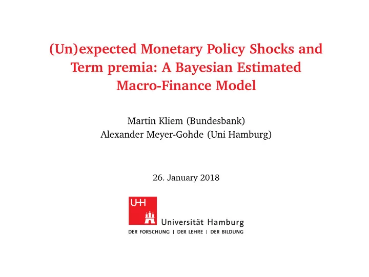
(Un)expected Monetary Policy Shocks and Term premia: A Bayesian Estimated Macro-Finance Model Martin Kliem (Bundesbank) Alexander Meyer-Gohde (Uni Hamburg) 26. January 2018

Disclaimer The views expressed in this presentation are those of the authors and do not reflect the opinions of the Deutsche Bundesbank. 1 / 23 Introduction Model Solution & Estimation Results Conclusion

Introduction Model Solution & Estimation Results Conclusion

Research Question What are the quantified effects of monetary policy on the term structure? ◮ Empirical literature has yet to reach a definitive conclusion ◮ Linear structural models do not go beyond expectation hypothesis ◮ Nonlinear structural models face significant quantitative constraints ⇒ To answer this question, we need a structural model which ◮ successfully explains macro and finance facts simultaneously ◮ allowing us to study different monetary policy tools ⇒ We analyze monetary policy in a workhorse New Keynesian model ◮ macros and yield curve estimated jointly with Bayesian likelihood ◮ underlying macro risks generate upward sloping yield via no- arbitrage pricing of risk 2 / 23 Introduction Model Solution & Estimation Results Conclusion

This paper estimates a structural model ...with time-variation in risk premia 7 Model Nominal 10−year term premium in % Corresponding estimates in the literature 6 5 4 3 2 1 0 1985 1990 1995 2000 2005 Figure : Model implied 10-year nominal term premium (black line) and range of corresponding estimates in the literature (gray area). 3 / 23 Introduction Model Solution & Estimation Results Conclusion

Main findings I ◮ Predicts upward sloping nominal and real yield curves ◮ Real risk premia play important role 70% real risk, 30% inflation risk → ◮ Historical smoothed time series for bonds and risk premia → comparable to empirical estimates 4 / 23 Introduction Model Solution & Estimation Results Conclusion

Some empirical evidence Hanson and Stein (2015): Monetary news has strong effects on forward real rates mostly reflecting change in the real term premia. Nakamura and Steinsson (2017): Monetary news has small effects on risk premia. Qualitative impact on nominal term premium depends on maturity Abrahams et al. (2016): Confirms findings from Hanson and Stein (2015); nominal term premium increases after increase of policy rate (see also Gertler and Karadi (2015)) Crump et al. (2016): Contrarily, decrease of nominal term premium after increase of policy rate = ⇒ Different samples, identification approaches, do not distinguish btw. forward guidance, systematic component, or shock to residual (see Ramey (2016)) 5 / 23 Introduction Model Solution & Estimation Results Conclusion

Main findings II ◮ A standard MP shock has small effects on term premium (see Naka- mura and Steinsson (2017)) ◮ A shock to the systematic component of MP has larger and long lasting effects on term premium (see Hanson and Stein (2015)) ◮ Unconditional forward guidance increases real and inflation risk of long-term bonds → Nominal term premium increases (see Akkaya et al. (2015)) which dampens the expansionary effect 6 / 23 Introduction Model Solution & Estimation Results Conclusion

Introduction Model Solution & Estimation Results Conclusion

Model overview ◮ general equilibrium macro-finance model (e.g. Rudebusch and Swanson (2012); Andreasen et al. (2017)) ◮ closed-economy New-Keynesian DSGE ◮ nominal and real frictions ◮ external habit formation ◮ long-run nominal and real risk ◮ price stickiness (Calvo) ◮ monetary policy characterized by Taylor-rule ◮ consumption-based asset pricing (arbitrage-free, frictionless) ⇒ we use recursive preferences (Epstein-Zin-Weil) to disentangle intertemporal elasticity of substitution and risk aversion 7 / 23 Introduction Model Solution & Estimation Results Conclusion

Monetary Policy Taylor-type policy rule: � � � y t r real + 4log π t + η y log 4 r f t = 4 · ρ R r f t − 1 + ( 1 − ρ R ) 4¯ z + t ¯ y � π 4 �� + η π log t + σ m ε m , t π ∗ t Time-varying inflation target (long–run nominal risk): log π ∗ t − 4log ¯ � log π ∗ t − 1 − 4log ¯ � + 4 ζ π ( log π t − 1 − log ¯ π = ρ π π π ) + σ π ε π , t 8 / 23 Introduction Model Solution & Estimation Results Conclusion

Bond pricing Nominal zero-coupon bond prices ( p ( 0 ) p ( 0 ) = 1 and ˆ = 1): t t � − 1 M t , t + 1 p ( n − 1 ) p ( n − 1 ) Risky: p ( n ) � � p ( n ) � R f � � , Risk neutral: ˆ ˆ = E t = E t t + 1 t + 1 t t t The continuously compounded return of n -period bond is defined as: = − 1 r ( n ) n log p ( n ) t t Term premium: difference between the risky and risk-neutral returns n − 1 TP ( n ) = 1 = − 1 � M t + j + 1 , p ( n − j − 1 ) � p ( n ) − log p ( n ) � � � log ˆ e − r t , t + j + 1 cov t + j nE t t + j + 1 t t n j = 0 9 / 23 Introduction Model Solution & Estimation Results Conclusion

Introduction Model Solution & Estimation Results Conclusion

Higher-order solution technique (see Meyer-Gohde (2016)) ◮ We adjust point and slope for risk out to second moments ◮ capture both constant and time-varying risk premium ◮ risk-sensitive linear approximation around the ergodic mean ⇒ non-certainty-equivalent approximation, but linear in states ⇒ This allows us to use the standard set of tools for estimation and analysis of linear models, without limiting the approximation to the certainty-equivalent approximation around the deterministic steady state. 10 / 23 Introduction Model Solution & Estimation Results Conclusion

Linear Non-Certainty Equivalent Approximation ◮ For the policy function y t = g ( y t − 1 , ǫ t , σ ) ◮ Reorganize partial derivatives at deterministic steady state � � y y i , ǫ j , σ k � � y = y , ǫ = 0, σ = 0 ◮ to construct approximations (in σ ) of ◮ ergodic mean y ( σ ) ≡ E [ g ( y t − 1 , σǫ t , σ )] = E [ y t ] ◮ derivatives at the ergodic mean y y ( σ ) ≡ g y ( y ( σ ) ,0, σ ) y ǫ ( σ ) ≡ g ǫ ( y ( σ ) ,0, σ ) ◮ Linear approximation at the (approximated) ergodic mean y t ≃ y ( σ ) + y y ( σ )( y t − 1 − y ( σ )) + y ǫ ( σ ) ǫ t Accuracy 11 / 23 Introduction Model Solution & Estimation Results Conclusion

Estimation ◮ We estimate the model using macro and financial data from 1983:Q1 until 2007:Q4 → Choice of time span driven by financial crisis starting in 2008 and change of systematic monetary policy at beginning of 1980s ◮ Macro data: real GDP growth ( ∆ y t ), real consumption growth ( ∆ c t ), real investment growth ( ∆ I t ), inflation ( π t ), policy rate ( R t , 3m T-bill) ◮ Survey data: 1q and 4q-ahead expected short rates ( E � � , E � � ) R t , t + 1 R t , t + 4 ◮ Financial data : US Treasury yields with 1year, 2year, 3year, 5year, and 10year maturity from Adrian et al (2013) ◮ We use an endogenous prior approach (Del Negro and Schorfheide, 2008) to explain key macro and asset pricing facts jointly Details ◮ Posterior estimates of parameters in line with other New Keynesian and macro-finance studies Estimates 12 / 23 Introduction Model Solution & Estimation Results Conclusion

Introduction Model Solution & Estimation Results Conclusion

Predicted nominal yield curve 7.5 7 Annualized Yields in % 6.5 6 5.5 5 Median Data 0 10 20 30 40 Maturity (Quarter) Figure : Nominal Yield Curve Why is the nominal yield curve upward sloping? 13 / 23 Introduction Model Solution & Estimation Results Conclusion

Predicted term structure of interest rates 7 200 6.5 Annualized Premia in Basis Points 6 Annualized Yields in % 150 5.5 5 4.5 100 4 3.5 50 3 Det. Steady State Det. Steady State 2.5 Median Median 0 0 10 20 30 40 0 10 20 30 40 Maturity (Quarter) Maturity (Quarter) (a) Real Yield Curve (b) Nominal Term Premium 160 70 140 Annualized Premia in Basis Points Annualized Premia in Basis Points 60 120 50 100 40 80 30 60 20 40 10 20 Det. Steady State Det. Steady State Median Median 0 0 0 10 20 30 40 0 10 20 30 40 Maturity (Quarter) Maturity (Quarter) (c) Real Term Premium (d) Inflation risk premium Why is the real yield curve upward sloping? 14 / 23 Introduction Model Solution & Estimation Results Conclusion

Predicted 1st and 2nd moments: macro variables Name Data Model Mean S.d. Mean S.d. GDP growth 0.540 0.593 0.803 0.540 [ 0.515,0.764 ] [ 0.761,0.838 ] Consumption growth 0.610 0.435 0.559 0.540 [ 0.383,0.515 ] [ 0.528,0.587 ] Investment growth 0.620 2.096 2.292 0.620 [ 1.796,2.744 ] [ 2.120,2.438 ] Annualized inflation 2.496 1.022 2.469 1.198 [ 0.840,1.493 ] [ 2.418,2.515 ] [ 1.136,1.254 ] Annualized policy rate 5.034 2.069 5.144 2.861 [ 1.521,3.927 ] [ 5.070,5.222 ] [ 2.733,3.026 ] Table : Predicted first and second moments of selected macro variables. Bold moments are calibrated. 15 / 23 Introduction Model Solution & Estimation Results Conclusion