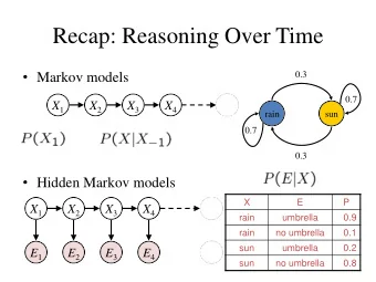
Umbrella World Suppose you are a security guard robot at an - PDF document

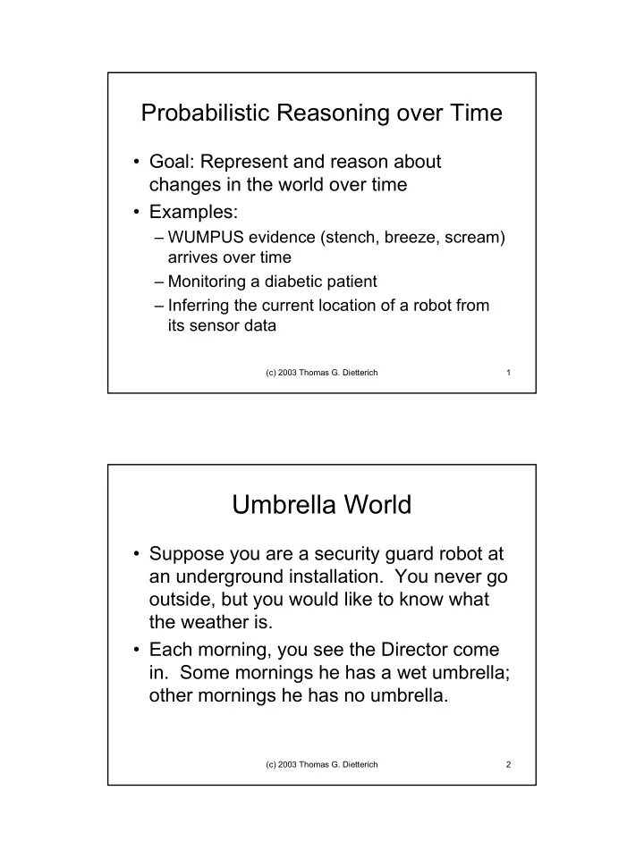
Probabilistic Reasoning over Time • Goal: Represent and reason about changes in the world over time • Examples: – WUMPUS evidence (stench, breeze, scream) arrives over time – Monitoring a diabetic patient – Inferring the current location of a robot from its sensor data (c) 2003 Thomas G. Dietterich 1 Umbrella World • Suppose you are a security guard robot at an underground installation. You never go outside, but you would like to know what the weather is. • Each morning, you see the Director come in. Some mornings he has a wet umbrella; other mornings he has no umbrella. (c) 2003 Thomas G. Dietterich 2 1

Notation • State variables (is it raining on day i?): R 0 , R 1 , R 2 , … • Evidence variables (is he carrying an umbrella on day i?): U 1 , U 2 , U 3 , … • X a:b denotes X a , X a+ 1 , …, X b-1 ,X b (c) 2003 Thomas G. Dietterich 3 Hidden Markov Model … R 0 R 1 R 2 R 3 R 4 R 5 R 6 R 7 U 1 U 2 U 3 U 4 U 5 U 6 U 7 • Markov assumption: P(R t |R 1:t-1 ) = P(R t |R t-1 ) Captures the “dynamics” of the world. For example, rainy days and non-rainy days come in “groups” • Sensor model: P(U t |R t ) • Stationarity: True for all times t (c) 2003 Thomas G. Dietterich 4 2

Probability Distributions R t R t-1 =no R t-1 =yes U t R t =no R t =yes no 0.7 0.3 no 0.8 0.1 yes 0.3 0.7 yes 0.2 0.9 0.3 no yes 0.7 0.7 0.3 We can view the HMM as a probabilistic finite state machine (c) 2003 Thomas G. Dietterich 5 Joint Distribution R 0 R 1 R 2 R 3 R 4 R 5 R 6 R 7 U 1 U 2 U 3 U 4 U 5 U 6 U 7 P(R 0:n ,U 0:n ) = P(R 0 ) ∏ t=1 P(R t |R t-1 ) · P(U t |R t ) Can be generalized to multiple state variables (e.g., position, velocity, and acceleration) and multiple sensors (e.g., motor speed, battery level, wheel shaft encoders) (c) 2003 Thomas G. Dietterich 6 3

Temporal Reasoning Tasks • Filtering or Monitoring : Compute the belief state given the history of sensor readings. P(R t |U 1:t ) • Prediction : Predict future state for some k > 0. P(R t+k |U 1:t ) • Smoothing : Reconstruct a previous state given subsequent evidence. P(R k |U 1:t ) • Most Likely Explanation : Reconstruct entire sequence of states given entire sequence of sensor readings. argmax R1:n P(R 1:n |U 1:n ) (c) 2003 Thomas G. Dietterich 7 Filtering by Variable Elimination P(R 1 |U 1 ) = Normalize[ ApplyEvidence[U 1 , ∑ R0 P(R 0 ) · P(R 1 |R 0 ) · P(U 1 |R 1 ) ] ] = Normalize[ ∑ R0 P(R 0 ) · P(R 1 |R 0 ) · P[R 1 ] ] = Normalize[ P[R 1 ] · ∑ R0 P(R 0 ) · P(R 1 |R 0 ) ] = Normalize[ P[R 1 ] · P[R 1 ] ] = Normalize[ P[R 1 ] ] P(R 2 |U 1:2 ) = Normalize[ ApplyEvidence[ U 1:2 , ∑ R0:1 P(R 0 ) · P(R 1 |R 0 ) · P(U 1 |R 1 ) · P(R 2 |R 1 ) · P(U 2 |R 2 ) ] ] = Normalize[ ∑ R0:1 P(R 0 ) · P(R 1 |R 0 ) · P[R 1 ] · P(R 2 |R 1 ) · P[R 2 ] ] = Normalize[ ∑ R1 [ ∑ R0 P(R 0 ) · P(R 1 |R 0 )] · P[R 1 ] · P(R 2 |R 1 ) · P[R 2 ] ] = Normalize[ [ ∑ R1 P[R 1 ] · P[R 1 ] · P(R 2 |R 1 )] · P[R 2 ] ] = Normalize[ P[R 2 ] · P[R 2 ]] = Normalize[ P[R 2 ] ] (c) 2003 Thomas G. Dietterich 8 4

General Pattern ∑ Rt-1 P(R t-1 |U 1:t-1 ) · P(R t |R t-1 ) · P(U t |R t ) Apply Evidence U t ∑ Rt-1 P[R t ] P[R t ] P[R t ] Influence of previous Influence of evidence time steps on R t U t on R t Normalize P(R t |U 1:t ) (c) 2003 Thomas G. Dietterich 9 The Forward Algorithm Define: Forward(P(R t-1 |U 1:t-1 ), Ut) = ∑ Rt-1 P(R t-1 |U 1:t-1 ) · P(R t |R t-1 ) · ApplyEvidence[U t , P(U t |R t )] Then filtering can be written recursively as: P(R t |U 1:t ) = Normalize[ Forward(P(R t-1 |U 1:t-1 ), U t )] In general, we can iterate over multiple time steps: Forward(P(R i |U 1:i-1 ), U i:t ) = Forward(Forward(P(R i |U 1:i-1 ), U i ), U i+1:t ) while i · t (c) 2003 Thomas G. Dietterich 10 5

Example: Day 1 • day 1: Umbrella. U 1 = yes P(R 1 ) = Normalize[Forward(P(R 0 ),yes)] R 0 P(R 0 ) R 1 R 0 =no R 0 =yes U 1 R 1 =no R 1 =yes . . Normalize [ ∑ R0 ] no 0.5 no 0.7 0.3 no 0.8 0.1 yes 0.5 yes 0.3 0.7 yes 0.2 0.9 R 1 R 0 =no R 0 =yes U 1 R 1 =no R 1 =yes . Normalize [ ∑ R0 ] no 0.7 * 0.5 0.3 * 0.5 no 0.8 0.1 yes 0.3 * 0.5 0.7 * 0.5 yes 0.2 0.9 (c) 2003 Thomas G. Dietterich 11 Example: Day 1 (continued) R 1 R 0 =no R 0 =yes U 1 R 1 =no R 1 =yes . Normalize [ ∑ R0 ] no 0.35 0.15 no 0.8 0.1 yes 0.15 0.35 yes 0.2 0.9 R 1 U 1 R 1 =no R 1 =yes . Normalize [ ] no 0.50 no 0.8 0.1 yes 0.50 yes 0.2 0.9 R 1 P(R 1 ) R 1 P(R 1 ) Normalize [ ] = no 0.18 no 0.10 yes 0.82 yes 0.45 (c) 2003 Thomas G. Dietterich 12 6

Example: Day 2 • Day 2: U 2 = yes R 2 R 1 =no R 1 =yes U 2 R 2 =no R 2 =yes R 1 P(R 1 ) . . ] Normalize [ ∑ R1 no 0.7 0.3 no 0.8 0.1 no 0.18 yes 0.3 0.7 yes 0.2 0.9 yes 0.82 R 2 R 1 =no R 1 =yes U 2 R 2 =no R 2 =yes . Normalize [ ∑ R1 ] no 0.7 * 0.18 0.3 * 0.82 no 0.8 0.1 yes 0.3 * 0.18 0.7 * 0.82 yes 0.2 0.9 R 2 R 1 =no R 1 =yes U 2 R 2 =no R 2 =yes . Normalize [ ∑ R1 ] = no 0.127 0.245 no 0.8 0.1 yes 0.055 0.573 yes 0.2 0.9 (c) 2003 Thomas G. Dietterich 13 Day 2 (continued) R 2 R 1 =no R 1 =yes U 2 R 2 =no R 2 =yes . Normalize [ ∑ R1 ] = no 0.127 0.245 no 0.8 0.1 yes 0.055 0.573 yes 0.2 0.9 R 2 U 2 R 2 =no R 2 =yes . ] = Normalize [ no 0.373 no 0.8 0.1 yes 0.627 yes 0.2 0.9 R 2 R 2 P(R 2 ) Normalize [ ] = no 0.075 no 0.116 yes 0.565 yes 0.883 (c) 2003 Thomas G. Dietterich 14 7

Prediction: Multiply by the Transition Probabilities and Sum Away • P(R t+k | U 1:t ) = ∑ Rt:t+k-1 P(R t | U 1:t ) · P(R t+1 |R t ) · P(R t+2 |R t+1 ) · … · P(R t+k |R t+k–1 ) • P(R t+1 | U 1:t ) = ∑ Rt P(R t | U 1:t ) · P(R t+1 |R t ) • P(R t+2 | U 1:t ) = ∑ Rt+1 P(R t+1 | U 1:t ) · P(R t+2 |R t+1 ) • … (c) 2003 Thomas G. Dietterich 15 Question: What Happens if We Predict Far Into the Future? • Each multiplication by P(R t+1 |R t ) makes our predictions “fuzzier”. Eventually, (for this problem) they converge to h 0.5,0.5 i . This is called the stationary distribution of the Markov process. Much is known about the stationary distribution and the rate of convergence. The stationary distribution depends on the transition probability distribution. (c) 2003 Thomas G. Dietterich 16 8

Smoothing: Reconstructing R k given U 1:t R 0 R 1 R 2 R 3 R 4 R 5 R 6 R 7 U 1 U 2 U 3 U 4 U 5 U 6 U 7 Forward � � Backward Assume k < t. Example: k=3, t=7: P(R 3 |U 1:7 ) = Normalize[ ApplyEvidence[U 1:7 , P(R 3 |U 1:3 ) · P(U 4:7 |R 3 ) ] ] (c) 2003 Thomas G. Dietterich 17 The Backward Algorithm ∑ Rt P(U t |R t ) · P(R t |R t-1 ) · P[R t ] Apply Evidence U t P[R t ] ∑ Rt P[R t-1 ] (c) 2003 Thomas G. Dietterich 18 9

The Backward Algorithm (2) Backward(P[R t ], U t )= ∑ Rt ApplyEvidence[U t , P(U t |R t )] · P(R t |R t-1 ) · P[R t ] This can then be applied recursively P[R t-1 ] = Backward(P[R t ], U t ) (c) 2003 Thomas G. Dietterich 19 Forward-Backward Algorithm for Smoothing R 0 R 1 R 2 R 3 R 4 R 5 R 6 R 7 U 1 U 2 U 3 U 4 U 5 U 6 U 7 Forward � � Backward P(R k |U 1:t ) = Normalize[ Forward(P(R 0 ), U 1:k ) · Backward(1, U k+1:t ) ] (c) 2003 Thomas G. Dietterich 20 10

Umbrella Example: P(R 1 |U 1:2 ) Normalize[ Forward(P(R 0 ), U 1 ) · Backward(1, U 2 ) ] R 1 P(R 1 ) Forward(P(R0), U1) = no 0.18 yes 0.82 Backward(1, U1) = ∑ R2 1 · P(R 2 |R 1 ) · P(U 2 |R 2 ) (c) 2003 Thomas G. Dietterich 21 Backward from Day 2 U 2 = yes R 2 P[R 2 ] R 2 R 1 =no R 1 =yes U 2 R 2 =no R 2 =yes . . ∑ R2 no 1 no 0.7 0.3 no 0.8 0.1 yes 1 yes 0.3 0.7 yes 0.2 0.9 R 2 R 1 =no R 1 =yes ∑ R2 no 0.7 * 1 * 0.2 0.3 * 1 * 0.2 yes 0.3 * 1 * 0.9 0.7 * 1* 0.9 R 2 R 1 =no R 1 =yes R 1 P[R 1 ] ∑ R2 = no 0.14 0.06 no 0.41 yes 0.27 0.63 yes 0.69 (c) 2003 Thomas G. Dietterich 22 11

Forward-Backward: R 1 P(R 1 ) R 1 P[R 1 ] . Normalize[ no 0.18 no 0.41 ] = yes 0.82 yes 0.69 R 1 P(R 1 ) R 1 P(R 1 ) Normalize[ no 0.074 ] = no 0.115 yes 0.566 yes 0.885 Notice that P(R 1 =yes|U 1 =yes) < P(R 1 =yes|U 1 =yes,U 2 =yes) Evidence from the future allows us to revise our beliefs about the past. (c) 2003 Thomas G. Dietterich 23 Most Likely Explanation • Find argmax R1:n P(R 1:n |U 1:n ) – Note that this is the maximum over all sequences of rain states: R 1:n – There are 2 n such sequences! – Fortunately, there is a dynamic programming algorithm: the Viterbi Algorithm (c) 2003 Thomas G. Dietterich 24 12

Viterbi Algorithm • Suppose we observe h yes,yes,no,yes,yes i for U 1:5 • Our goal is to find the best path through a “trellis” of possible rain states: (c) 2003 Thomas G. Dietterich 25 Max distributes over conformal product B A=no A=yes C B=no B=yes . max A,B,C no 0.10 0.20 no 0.10 0.35 = yes 0.40 0.15 yes 0.30 0.40 B C A=no A=yes B C A=no A=yes no no 0.10*0.10 0.20*0.10 no no 0.010 0.020 no yes 0.10*0.40 0.20*0.40 = no yes 0.040 0.080 yes no 0.30*0.35 0.40*0.35 yes no 0.105 0.140 yes yes 0.30*0.15 0.40*0.15 yes yes 0.045 0.060 (c) 2003 Thomas G. Dietterich 26 13