Turbulence on APE: towards channel@apeNEXT GGI Firenze 2007 - PowerPoint PPT Presentation
Turbulence on APE: towards channel@apeNEXT GGI Firenze 2007 Federico Toschi IAC-CNR http://www.iac.cnr.it/~toschi The past, the present and the future APE100 RB, Channel flow APEmille RB, Channel flow, Fast Fourier
Turbulence on APE: towards channel@apeNEXT GGI Firenze 2007 Federico Toschi IAC-CNR http://www.iac.cnr.it/~toschi
The past, the present and the future • APE100 – RB, Channel flow • APEmille – RB, Channel flow, Fast Fourier Transform • apeNEXT – RB, Channel flow, Lagrangian Turbulence, – Microfluidic ?
Introduction to turbulence • What is fluid dynamics turbulence?? – Deterministic, non-linear & chaotic system. – Characterized by an infinite number of active degrees of freedom, in the infinite Re number limit (field theory) • Navier-Stokes is an open problem for math, physics, engineering (more later).
Navier-Stokes equations/turbulence + boundary conditions Inertial range Richardson cascade picture Typical feature: intermittency
Statistical observables in turbulence Structure functions : Well known, structure function behaviour, in the inertial range, for homogeneous and isotropic turbulence: With famous Kolmogorov’s prediction 1941: Exact result for homogeneous/isotropic turbulence:
Turbulence, a challenge for: • Mathematics – Existence of NS solutions. • Physics – How to compute anomalous scaling exponents ? (exponents = quantification of intemittency) – Universality issue ! • Engineering – Ability to simulate or reproduce realistic systems. • Computer science – Efficient computational methods.
The method of choice on APE: LBE Stream and collide Particularly tailored to APE topology
Boundary conditions for LBE code BC: good for APE easy, local, overlap communications & comp. BC: good for physics LBE scheme allow a big flexibility in bc !!! No slip Free slip Illustration of population injection from the “buffer” layer
What have we done with this ?
RB cell & plumes Pisa - APEmille Lyon - Nikon D70
Motivation Hot topics (still open today!): •Scaling of Nu vs. Ra and Pr •Bolgiano scaling and in particular on the statistics of velocity, temperature fields
What we studied over the years… – Studied several variants of convective cell (also periodic case !!) – Always cubic geometry – With different boundary conditions !! – Modest resolutions i.e. 160 3 and 240 3 – Very high statistics (i.e. hundreds of eddy turnover times)
Bolgiano scaling Boussinesq equations: Temperature difference Cell’s heigth Bolgiano scaling Kolmogorov scaling
The standard RB cell and L B (z) We introduced the “local” Bolgiano length From measuring this quantity one can understand how strongly non homogeneous a convective cell is R. Benzi, F. Toschi, R. Tripiccione On the Heat Transfer in Rayleigh-Bénard systems Journal of Statistical Physics 93 3 (1998)
The homogeneous Rayleigh-Bénard cell Where do the eqns. of HRB comes from? Here some more details... From Boussinesq approximation: Supposing temperature is the sum of a linear profile, plus fluctuating part: with one ends up with: Supplemented with periodic boundary conditions in all directions
Inside the HRB cell... • The system auto-mantains itself: no external forcing! • No boundary layers ! (see Lohse & Toschi PRL 2003) • The system is fully homogeneous BUT not isotropic • L B too big to see Bolgiano scaling Thermal plume Notice that the cell is fully periodic
Results from the standard cell
Bolgiano scaling maybe close to walls From the behaviour of L B one learns that to see Bolgiano scaling one has to move close to the top/bottom isothermal walls Is this enough? Is it so simple? What happens near to the walls (inside a boundary layers) ?
The boundary layer problem Structure functions from a boundary layer experiment Slope 1 Slope gets smaller and smaller than 1 moving near to the walls
The boundary layer problem Slope 2 Slope 1.78 Slope 1 Structure functions of order 3 and 6 at y + =102 from a boundary layer experiment
How to get the scaling exponents Problem: resolution too small for scaling in real space
Exponents from the standard cell Scaling exponents for velocity and temperature Consistent with Bolgiano scaling !!
Results from the homogeneous cell
Ultimate regime for RB ...idea. Use the homogenous cell to check the Kraichnan regime: R. H. Kraichnan, Phys. Fluids 5, 1374 (1962) Prediction: results from our DNS...
Nu and Re vs. Ra
Channel flow: non homogeneous turb.
Turbulent cascade: L 0 -> η Energy flux Inertial range
Idealized turbulence: H/I Exact relation for homogeneous and isotropic turbulence Exact result for homogeneous/isotropic turbulence: What about fluctuations ? Fluctuations intermittent very complicated but the following remarkable relation holds for any inertial distance, r, Refined Kolmogorov Similarity Hypothesis RKSH
Eddy viscosity is a crazy idea • Large eddy simulation: resolve only scales larger than • Eddy viscosity: model the subgrid scales in terms of a cutoff dependent effective viscosity (unresolved scales act on resolved ones through a renormalized “eddy” viscosity)
Eddy viscosity If such an eddy viscosity exist it must be able to “eat” the energy flux Definition of eddy viscosity RKSH RKSH -> Smagorinsky
Boundary layer Turbulence Surprise ! First flow where violations to RKSH has been reported
Non ideal turbulence: boundary layers
Mapping non ideal on ideal turbulence Also change of the RKSH
Results from experimental boundary layer from exp… from APE100… Compensated structure functions for several orders
Eddy viscosity in presence of shear In general, in presence of shear: Definition of eddy viscosity RKSH Generalized RKSH -> SISM
Shear Improved Smagorinsky Model (SISM) SISM model:
Test of the SISM 1) Spectral channel flow 2) Finite difference backward facing step
Average profiles
Reynolds stress
Lagrangian turbulence
Roadmap
Any realistic approach to Lagrangian turbulence requires going through (at least) the following steps: • Neutrally buoyant case Realistic flow geometries – Smaller that the dissipative scale of turbulence and with same density of advecting field • Heavy particle case – Smaller that the dissipative scale of turbulence but with density much higher that advecting field – One way coupling – Two way coupling • Generic density contrast case We are here… – One way coupling – Two way and four way coupling (collisions) • Non idealized particles – Finite particle size, non spherical geometry case, etc… • Thermal effects (both stable and unstable conditions) • Intrinsic dynamics (i.e.droplest in clouds) – Radii growth – Coalescence, etc…
Will present two cases: Lagrangian tracers (i.e. pointwise, neutrally buoyant particles) Heavy particles (i.e. particle density much larger than fluid density)
Equation of motion for Lagrangian Tracers The simplest case of Lagrangian turbulence is the evolution of small (infinitesimal) fluid elements. This is equivalent to the evolution of very small particles with density matched with that of the advecting turbulent field. Starting position Starting time Eulerian advecting turbulent field
Equation of motion for “real” particles Maxey, M. & Riley, J. 1983 Equation of motion of a small rigid sphere in a nonuniform flow. Phys. Fluids 26, 883-889. Maxey, M. & Riley, J. 1983 Equation of motion of a small rigid sphere in a nonuniform flow. Phys. Fluids 26, 883-889. Stokes number
Experimental state of the art Experimental Lagrangian measurements are intrinsically difficult: one has to follow (many) Lagrangian trajectories for long time at high Reynolds (i.e. high sampling frequency) Ott and Mann experiment at Risø Bodenschatz experiment at Cornell conventional 3D PTV - Re λ =100 (now Re λ ≈ 300) fast silicon strip detectors (now fast CCD cameras) Re λ ≈ 1000-1500 Pinton experiment at ENSL ultrasonic Doppler tracking - Re λ =740 (single particle tracking)
Lagrangian Tracers integration δ x η τ η N Re λ L T L T N p 512 183 0.01 3.14 2.1 0.048 5 0.012 0.96 10 6 1024 284 0.005 3.14 1.8 0.033 4.4 0.006 1.92 10 6 Pseudo spectral code - dealiased 2/3 rule - normal viscosity - 2 millions of passive tracers- code fully parallelized with Energy spectrum MPI+FFTW - Platform IBM SP4 (sust. Performance 150Mflops/proc) - duration of the run: 40 days k -5/3 Spectral flux Lagrangian database (x(t),v(t),a(t)=- ∇ p+ ν � u) at high resolution
Heavy particles - Lagrangian integration L3 2563 5123 Total particles 32 Mparticles 120 Mparticles Stokes/ LyapStokes 16/32 16/32 Slow dumps 10 2.000.000 7.500.000 Fast dumps 0.1 250.000 500.000 8 10-4 4 10-4 dt Time step ch0+ch1 756 + 1744 900 + 2100 τ η 0.0746 0.0466 0.0, 0.00753454, 0.0125576, 0.0175806, 0.0226036, 0.0, 0.0120, 0.0200, 0.0280, 0.0360, 0.0440, 0.0520, τ 0.0276266, 0.0326497, 0.0376727, 0.0426957, 0.0600, 0.0680, 0.0760, 0.0840, 0.1000, 0.1200, 0.152, 0.0477187, 0.0527418, 0.0627878, 0.0753454, 0.200, 0.248 0.0954375, 0.125576, 0.155714 Disk space used 400 GByte 1 TByte
Recommend
More recommend
Explore More Topics
Stay informed with curated content and fresh updates.
