Topic 6: 3D Curves Intro to curve interpolation & approximation - PowerPoint PPT Presentation
Topic 6: 3D Curves Intro to curve interpolation & approximation Polynomial interpolation Bzier curves Cardinal splines Interactive Design of Curves Goal: Expand the capabilities of shapes beyond lines and conics, simple
Topic 6: 3D Curves • Intro to curve interpolation & approximation • Polynomial interpolation • Bézier curves • Cardinal splines
Interactive Design of Curves Goal: Expand the capabilities of shapes beyond lines and conics, simple analytic functions and to allow design constraints. Design Issues: • Continuity (smoothness) • Control (local vs. global) • Interpolation vs. approximation of constraints • Other geometric properties (planarity, tangent/curvature control) • Efficient analytic representation
Parametric Polynomial Curves Recall a linear curve (line) is: p(t) = a 1 t+a 0 A cubic curve is similarly: …or p(t) = d 3 t 3 +d 2 t 2 +d 1 t+d 0 , where d i = [a i , b i , c i ,] T Cubics are commonly used in graphics because curves of lower order commonly have too little flexibility (only planar, no curvature control), while curves of higher order are unnecessarily complex and make it easy to introduce undesired wiggles.
Designing Polynomial Curves from constraints p(t) = TA , where T is powers of t. for a cubic T=[t 3 t 2 t 1 1]. Written with geometric constraints p(t) = TMG, where M is the Basis matrix of a design curve and G the specific design constraints. An example of constraints for a cubic Hermite for eg. are end points and end tangents. i.e. P 1 ,R 1 at t=0 and P 4 ,R 4 at t=1. Plugging these constraints into p(t) = TA we get. B p(0) = P 1 = [ 0 0 0 1 ] A h p(1) = P 4 = [ 1 1 1 1 ] A h => G=BA, A=MG => M=B -1 p'(0)= R 1 = [ 0 0 1 0 ] A h p'(1)= R 4 = [ 3 2 1 0 ] A h
Hermite Basis Matrix An example of constraints for a cubic Hermite for eg. are end points and end tangents. i.e. P 1 ,R 1 at t=0 and P 4 ,R 4 at t=1. Plugging these constraints into p(t) = TA we get. B p(0) = P 1 = [ 0 0 0 1 ] A h p(1) = P 4 = [ 1 1 1 1 ] A h => G=BA, A=MG => M=B -1 p'(0)= R 1 = [ 0 0 1 0 ] A h p'(1)= R 4 = [ 3 2 1 0 ] A h
Hermite Basis Matrix [ 0 0 0 1 ] -1 [ 1 1 1 1 ] [ 0 0 1 0 ] [ 3 2 1 0 ] = M hermite [ 2 -2 1 1 ] [ -3 3 -2 -1 ] [ 0 0 1 0 ] [ 1 0 0 0 ]
Catmull-Romm splines using Hermite curves Catmull-Romm Interpolation p 3 p 1 p 0 p 4 p 2 Pick tangents based on a factor k (1/2 for eg.) of the vector between neighbor points. p’ i = k*(p i+1 - p i-1 ). For the end-points there is only one neighbor: p’ 0 = k*(p 1 - p 0 ). p’ n = k*(p n – p n-1 ).
Bezier Basis Matrix A cubic Bezier can be defined with four points where: P 1 ,R 1 at t=0 and P 4 ,R 4 at t=1 for a Hermite. R 1 = 3(P 2 -P 1 ) and R 4 = 3(P 4 -P 3 ). We can thus compute the Bezier Basis Matrix by finding the matrix that transforms [P 1 P 2 P 3 P 4 ] T into [P 1 P 4 R 1 R 4 ] T i.e. B_H =[ 1 0 0 0 ] [ 0 0 0 1] [-3 3 0 0] [ 0 0 -3 3] M bezier =M hermite * B_H
Bezier Basis Functions [ -1 3 -3 1 ] [ 3 -6 3 0 ] [ -3 3 0 0 ] [ 1 0 0 0 ] The columns of the Basis Matrix form Basis Functions such that: p(t)= f 1 (t)P 1 + f 2 (t)P 2 + f 3 (t)P 3 + f 4 (t)P 4. From the matrix: n ) * (1-t) (n-i) * t i f i (t) = ( i These are also called Bernstein polynomials.
Bezier Basis Functions [ -1 3 -3 1 ] [ 3 -6 3 0 ] [ -3 3 0 0 ] [ 1 0 0 0 ] The columns of the Basis Matrix form Basis Functions such that: p(t)= f 1 (t)P 1 + f 2 (t)P 2 + f 3 (t)P 3 + f 4 (t)P 4. From the matrix: n ) * (1-t) (n-i) * t i f i (t) = ( i These are also called Bernstein polynomials.
Basis Functions Basis functions can be thought of as interpolating functions. Note: actual interpolation of any point only happens if its Basis function is 1 and all others are zero at some t. Often Basis functions for design curves sum to 1 for all t. This gives the curve some nice properties like affine invariance and the convex hull property when the function are additionally non-negative.
Geometric continuity at a joint of two curves Geometric Continuity G 0 : curves are joined G 1 : first derivatives are proportional at the join point The curve tangents thus have the same direction, but not necessarily the same magnitude. i.e., C 1 '(1) = (a,b,c) and C 2 '(0) = (k*a, k*b, k*c). G 2 : first and second derivatives are proportional at join point Parametric Continuity C 0 : curves are joined C 1 : first derivatives equal C 2 : first and second derivatives are equal If t is taken to be time, the acceleration is continuous. C n : nth derivatives are equal
Local vs. Global control Changing a point on the Bezier changes the curve mostly n ear the point, but a little bit everywhere… Precise local control can be handled by splines where the Basis functions of points symmetrically increase from 0 to a maximum value over a window and then decrease to 0. The curve is strictly affected by the point over this parameter range or window.
Recommend
More recommend
Explore More Topics
Stay informed with curated content and fresh updates.


