Too interconnected to fail: Contagion and Systemic Risk in Financial - PowerPoint PPT Presentation
Too interconnected to fail: Contagion and Systemic Risk in Financial Networks Rama CONT Joint work with: Amal Moussa ( Columbia University) Andreea Minca (Universit e de Paris VI) Edson Bastos (Banco Central do Brasil) 1 Financial
Too interconnected to fail: Contagion and Systemic Risk in Financial Networks Rama CONT Joint work with: Amal Moussa ( Columbia University) Andreea Minca (Universit´ e de Paris VI) Edson Bastos (Banco Central do Brasil) 1
Financial stability and systemic risk The recent financial crisis has simultaneously underlined the importance of contagion and systemic risk and the lack of adequate indicators for measuring and monitoring them. Control over systemic risk has been the main motivation of the recent bailouts of large financial institutions Regulators have had great difficulties anticipating the impact of defaults partly due to a lack of visibility and lack of relevant indicators on the structure of the financial system Policy has been guided by “too big to fail” principle Availability of better indicators of systemic risk would have greatly helped regulatory and crisis management policy. 2
A need for indicators of systemic impact ∙ US Treasury has called “for new legislation granting additional tools to address systemically significant financial institutions” (Mar 2009). ∙ The new legislation ” would cover financial institutions that have the potential to pose systemic risks to our economy”. ∙ “In determining whether to use the program for an institution,Treasury may consider the extent to which destabilization of the institution could threaten the viability of creditors and counterparties exposed to the institution whether directly or indirectly .” ∙ What makes an institution systematically significant”? ∙ Need for indicators of systemic impact of the failure of a financial institution 3
OBJECTIVES In this work we ∙ propose a quantitative approach for measuring the systemic impact of the failure of a large financial institution: the Systemic Risk Index ∙ This index combines the effects of – common market factors affecting defaults – default contagion via counterparty risk – indirect contagion via credit default swaps ∙ use this measure of systemic risk on empirical data and simulated network structures to study the influence of network structure, credit default swaps and clearinghouses on systemic risk in the banking system. 4
Systemic vs marginal risk ∙ Bank regulation has focused on the risk of individual financial institutions (VaR) to determine capital requirements ∙ Capital should be sufficient to cover typical losses of large magnitude ∙ VaR of an institution measures how much the institution can be harmed by market moves: it is concerned with the marginal loss distribution of the institutions portfolio ∙ On the contrary, systemic risk is concerned with how much the financial system can be harmed by the failure of the institution ∙ It is concerned with the joint distribution of the losses of all market participants and requires modeling how losses are transmitted through the financial system 5
LTCM ∙ LTCM: daily VaR= 400 million $ in Aug 1998, Size= 410 9 $. ∙ Amaranth: size = 9.5 billion USD. ∙ The default of Amaranth hardly made headlines: no systemic impact. ∙ The default of LTCM threatened the stability of the US banking system → Fed intervention ∙ Reason: LTCM had many counterparties in the world banking system, with large liabilities/exposures. ∙ Point 1 : Systemic impact/ default contagion is not about the size of a firm ∙ Point 2 : a firm’s portfolio can be “well-hedged” (low market risk using conventional measures) but the firm can be a source of large systemic risk 6
The network approach to contagion modeling We model a network of counterparty relations as a weighted directed graph whose ∙ 𝑜 vertices (nodes) 𝑗 ∈ 𝑊 represent financial market participants: banks, funds, corporate borrowers and lenders, hedge funds, insurers, monolines. ∙ (directed) links represent counterparty exposures: 𝑀 𝑗𝑘 is the the (market) value of liabilities of 𝑗 towards 𝑘 , 𝑀 𝑘𝑗 is the exposure of 𝑗 to 𝑘 . ∙ In a market-based framework 𝑀 𝑘𝑗 is understood as the fair market value of the exposure of 𝑗 to 𝑘 . ∙ Each institution 𝑗 disposes of a capital buffer 𝑑 𝑗 for absorbing market losses. In practice: Tier I+II capital minus required capital for non-banking assets. 7
∙ Solvency condition: 𝑑 𝑗 + ∑ 𝑘 𝑀 𝑘𝑗 − ∑ 𝑘 𝑀 𝑗𝑘 > 0 ∙ Capital absorbs first losses. Default occurs if Loss(i) > 𝑑 𝑗 . Assets Liabilities Interbank assets Interbank liabilities ∑ ∑ 𝑘 𝑀 𝑘𝑗 𝑘 𝑀 𝑗𝑘 Other Capital assets 𝐵 𝑗 𝐷 𝑗 Table 1: Stylized balance sheet of a bank. 8
Brazil’s interbank network Joint work with Edson BASTOS, Banco Central do Brasil. Data from 2008 provided by Bank of Brazil. ∙ Complete data set of all consolidated interbank exposures (including swaps)+ Tier I and Tier II capital. ∙ 𝑜 ≃ 100 institutions (holdings), ≃ 1000 counterparty relations ∙ Average number of counterparties (degree)= 7 ∙ In-degree (number of debtors) has a Pareto distribution with exponent ≃ 2. ∙ Out-degree (number of creditors) has a Pareto distribution with exponent ≃ 3. ∙ Exposures sizes very heterogeneous: heavy tailed distribution, a handful of bilateral exposures are > 100 times larger than most of the rest. 9
Figure 1: Brazilian interbank network (Cont & Bastos 2009). 10
Distribution of the Degree 5 4.5 4 3.5 3 2.5 2 1.5 1 0.5 0 0 50 100 150 Rank Figure 2: Brazilian interbank network: distribution of degree (num- ber of counterparties). 11
Distribution of the Out Degree 2 10 −2 −2.5 −3 −3.5 1 10 −4 −4.5 −5 −5.5 0 10 −6 0 50 100 150 0 1 2 3 Rank Figure 3: Brazilian interbank network: distribution of in-degree (number of creditors): Pareto tail with tail index ≃ 1.7 12
Distribution of In Degree Brazilian interbank exposures Dec 2008 2 10 0 −10 −20 1 10 −30 −40 −50 0 10 −60 0 50 100 150 0 5 10 15 20 25 Rank Figure 4: Brazilian interbank network: distribution of out-degree (number of debtors): Pareto tail with tail index ≃ 3 13
Distribution of the clustering coefficient 1 0.9 0.8 0.7 0.6 0.5 0.4 0.3 0.2 0.1 0 0 0.2 0.4 0.6 0.8 1 Clustering coefficient Figure 5: Brazilian interbank network: distribution of clustering coefficient 14
2 10 Degree 1 10 0 10 0 0.2 0.4 0.6 0.8 1 Clustering coefficient Figure 6: Brazilian interbank network: degree vs clustering coeffi- cient. 15
10 12000 10 10000 8000 6000 4000 2000 9 0 10 0.2 0.4 0.6 0.8 1 2 3 4 5 6 7 8 10 10 10 10 Figure 7: Rank diagram of largest counterparty exposures of AIG in Sept 2008 exhibits a similar Pareto tail. 16
A preferential attachment model for banking networks The graph 𝐻 ( 𝑢 ) is constructed iteratively in 𝑢 steps starting from an initial node. At step 𝑢 + 1 ∙ with probability 1 > 𝑞 > 0, add a new vertex v together with an edge from v to an existing vertex w chosen with probability 𝑒𝑓 in ( 𝑥 ) + 𝜀 in (1) . ∑ ∣ 𝐻 ( 𝑢 ) ∣ 𝑗 =1 ( 𝑒𝑓 in ( 𝑗 ) + 𝜀 in ) ∙ With probability 𝑞 , add a new vertex w and an edge from an existing vertex v to w, where v is chosen with probability 𝑒𝑓 out ( 𝑥 ) + 𝜀 out (2) . ∑ ∣ 𝐻 ( 𝑢 ) ∣ 𝑗 =1 ( 𝑒𝑓 out ( 𝑗 ) + 𝜀 out ) ∙ With probability 1 − 2 𝑞 , link an existing vertex v to an existing vertex w, where v and w are chosen independently, v with 17
probability (2) and w with probability (1). The construction is stopped when ∣ 𝐻 ( 𝑢 ) ∣ = 𝑂 . Interpretation: a new firm entering the financial system is more likely to establish financial links with highly connected firms. Once the graph is constructed we allocate IID exposures (weights) to each link with a Pareto distribution with exponent 2. 18
Property 1 (Degree distributions) . With probability 1, we have 1 𝑏.𝑡. 𝑂 # { 𝑤 ∈ [ 𝐻 𝑂 ] , 𝑗𝑜𝑒𝑓 ( 𝑤 ) = 𝑙 } → 𝑟 in ( 𝑙 ) (3) 1 𝑏.𝑡. 𝑂 # { 𝑤 ∈ [ 𝐻 𝑂 ] , 𝑝𝑣𝑢𝑒𝑓 ( 𝑤 ) = 𝑙 } → 𝑟 out ( 𝑙 ) (4) as 𝑂 → ∞ . Furthermore there exists constants 𝐷 in , 𝐷 out > 0 such that 𝐷 in 𝑙 →∞ 𝑟 out ( 𝑙 ) ∼ 𝑙 →∞ 𝐷 out 𝑟 in ( 𝑙 ) ∼ (5) 𝑙 𝛽 out 𝑙 𝛽 in with 𝛽 in = 2 − 𝑞 + 2 𝑞𝜀 in 𝛽 out = 2 − 𝑞 +2 𝑞𝜀 out (6) 1 − 𝑞 1 − 𝑞 In particular choosing 𝑞 = 0 . 1 , 𝜀 𝑗𝑜 = 0 , 𝜀 𝑝𝑣𝑢 = 4 . 45 we obtain 𝛽 in = 2 . 1 𝛽 out = 3 . 1 19
Distribution of the Out Degree (b) and In degree (r) 0 10 −1 10 −2 10 −3 10 0 1 2 3 10 10 10 10 Log scale Figure 8: Degree distributions obtained for random attachment model. In-exponent: 2.1; Out-exponent: 3 20
Distribution of the clustering coefficient 3 1 10 0.9 0.8 0.7 2 10 0.6 Degree 0.5 0.4 1 10 0.3 0.2 0.1 0 0 10 0 0.2 0.4 0.6 0.8 1 0 0.2 0.4 0.6 0.8 1 Clustering coefficient Clustering coefficient Figure 9: Left: distribution of clustering coefficient. Right: cluster- ing coefficient vs degree. 21
Recommend
More recommend
Explore More Topics
Stay informed with curated content and fresh updates.
