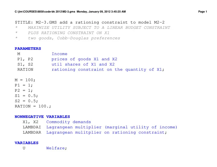

C:\jim\COURSES\8858\code-bk 2012\M2-3.gms Monday, January 09, 2012 3:45:25 AM Page 1 $TITLE: M2-3.GMS add a rationing constraint to model M2-2 * MAXIMIZE UTILITY SUBJECT TO A LINEAR BUDGET CONSTRAINT * PLUS RATIONING CONSTRAINT ON X1 * two goods, Cobb-Douglas preferences PARAMETERS M Income P1, P 2 prices of goods X1 and X2 S1, S 2 util shares of X1 and X2 R A T I O N rationing constraint on the quantity of X1; M = 100; P1 = 1; P2 = 1; S1 = 0.5; S2 = 0.5; RATION = 100.; NONNEGATIVE VARIABLES X1, X 2 Commodity demands L A M B D A I Lagrangean multiplier (marginal utility of income) L A M B D A R Lagrangean mulitplier on rationing constraint; VARIABLES U Welfare;
C:\jim\COURSES\8858\code-bk 2012\M2-3.gms Monday, January 09, 2012 3:45:25 AM Page 2 EQUATIONS U T I L I T Y Utility I N C O M E Income-expenditure constraint R A T I O N 1 Rationing contraint on good X1 FOC1, F O C 2 First-order conditions for X1 and X2; UTILITY.. U =E= 2*(X1**S1)*(X2**S2); INCOME.. M =G= P1*X1 + P2*X2; RATION1.. RATION =G= X1; FOC1.. LAMBDAI*P1 + LAMBDAR =G= 2*S1*X1**(S1-1)*(X2**S2); FOC2.. LAMBDAI*P2 =G= 2*S2*X2**(S2-1)*(X1**S1); * modeled as a non-linear programming problem * set starting values U.L = 100; X1.L = 50; X2.L = 50; LAMBDAI.L = 1; LAMBDAR.L = 0; MODEL OPTIMIZE /UTILITY, INCOME, RATION1/;
C:\jim\COURSES\8858\code-bk 2012\M2-3.gms Monday, January 09, 2012 3:45:25 AM Page 3 SOLVE OPTIMIZE USING NLP MAXIMIZING U; * modeled as a complementarity problem MODEL COMPLEM /UTILITY.U, INCOME.LAMBDAI, RATION1.LAMBDAR, FOC1.X1, FOC2.X2/; SOLVE COMPLEM USING MCP; * try binding rationing constraint at X1 <= RATION = 25; RATION = 25; SOLVE OPTIMIZE USING NLP MAXIMIZING U; SOLVE COMPLEM USING MCP; * show that shadow price of rationing constraint increases with income * could lead to a black market in rationing coupons, "scalping" tickets M = 200; SOLVE OPTIMIZE USING NLP MAXIMIZING U; SOLVE COMPLEM USING MCP; * illustrate the mpec solver * suppose we want to enforce the rationing contraint via licenses for X1 * consumers are given an allocation of licenses which is RATION
C:\jim\COURSES\8858\code-bk 2012\M2-3.gms Monday, January 09, 2012 3:45:25 AM Page 4 * PLIC is an endogenous variables whose value is the license price * the value of the rationing license allocation should be treated as * part of income NONNEGATIVE VARIABLES PLIC; EQUATIONS INCOMEa FOC1a; M = 100; RATION = 25; U.L = 100; X1.L = 25; X2.L = 75; PLIC.L = 0.1; INCOMEa.. M + (PLIC*RATION) =E= (P1 + PLIC)*X1 + P2*X2 ; FOC1a.. LAMBDAI*(P1 + PLIC) =G= 2*S1*X1**(S1-1)*(X2**S2); MODEL M P E C /UTILITY, INCOMEa.LAMBDAI, FOC1a.X1, FOC2.X2, RATION1.PLIC/; MODEL COMPLEM2 /UTILITY.U, INCOMEa.LAMBDAI, FOC1a.X1, FOC2.X2,
C:\jim\COURSES\8858\code-bk 2012\M2-3.gms Monday, January 09, 2012 3:45:25 AM Page 5 RATION1.PLIC/; OPTION MPEC = nlpec; SOLVE MPEC USING MPEC MAXIMIZING U; SOLVE COMPLEM2 USING MCP; M = 200; SOLVE MPEC USING MPEC MAXIMIZING U; SOLVE COMPLEM2 USING MCP; * now use the expenditure function, giving the minimum cost of buying * one unit of utility: COSTU = P1**S1 * P2**S2 = PU * where PU is the "price" of utility: the inverse of lambda * two versions are presented: * one using Marshallian (uncompensated) demand: Xi = F(P1, P2, M) * one using Hicksian (compensated) demand: Xi = F(P1, P2, U) RATION = 100; M = 100; NONNEGATIVE VARIABLES P U price of utility M 1 income inclusive of the value of rationing allocation;
C:\jim\COURSES\8858\code-bk 2012\M2-3.gms Monday, January 09, 2012 3:45:25 AM Page 6 EQUATIONS C O S T U expenditure function: cost of producing utility = PU D E M A N D M 1 Marshallian demand for good 1 D E M A N D M 2 Marshallian demand for good 2 D E M A N D H 1 Hicksian demand for good 1 D E M A N D H 2 Hicksian demand for good 2 D E M A N D U Demand for utility (indirect utility function) R A T I O N 1 b Rationing constraint (same as before) I N C O M E b Income balance equation; COSTU.. (PLIC+P1)**S1 * P2**S2 =G= PU; DEMANDM1.. X1 =G= S1*M1/(P1+PLIC); DEMANDM2.. X2 =G= S2*M1/P2; DEMANDH1.. X1 =G= S1*PU*U/(P1+PLIC); DEMANDH2.. X2 =G= S2*PU*U/P2; DEMANDU.. U =E= M1/PU; RATION1b.. RATION =G= X1; INCOMEb.. M1 =E= M + PLIC*RATION;
C:\jim\COURSES\8858\code-bk 2012\M2-3.gms Monday, January 09, 2012 3:45:25 AM Page 7 PU.L = 1; MODEL COMPLEM3 /COSTU.U, DEMANDM1.X1, DEMANDM2.X2, DEMANDU.PU, RATION1b.PLIC, INCOMEb.M1/; MODEL COMPLEM4 /COSTU.U, DEMANDH1.X1, DEMANDH2.X2, DEMANDU.PU, RATION1b.PLIC, INCOMEb.M1/; SOLVE COMPLEM3 USING MCP; SOLVE COMPLEM4 USING MCP; * counterfactuals RATION = 25; SOLVE COMPLEM3 USING MCP; SOLVE COMPLEM4 USING MCP; M = 200; SOLVE COMPLEM3 USING MCP; SOLVE COMPLEM4 USING MCP; *$exit
C:\jim\COURSES\8858\code-bk 2012\M2-3.gms Monday, January 09, 2012 3:45:25 AM Page 8 * scenario generation SETS I indexes different values of rationing constraint /I1*I10/ J indexes income levels /J1*J10/; PARAMETERS RLEVEL(I) PCINCOME(J) LICENSEP(I,J); U.L = 50; X1.L = 25; X2.L = 25; PLIC.L = 0.; LAMBDAI.L = 1; * the following is to prevent solver failure when evaluating X1**(S1-1) * at X1 = 0 (given S1-1 < 0) X1.LO = 0.01; X2.LO = 0.01; LOOP (I, LOOP (J, RATION = 110 - 10* ORD (I); M = 25 + 25* ORD (J);
C:\jim\COURSES\8858\code-bk 2012\M2-3.gms Monday, January 09, 2012 3:45:25 AM Page 9 SOLVE MPEC USING MPEC MAXIMIZING U; RLEVEL(I) = RATION; PCINCOME(J) = M; LICENSEP(I,J) = PLIC.L; ); ); DISPLAY RLEVEL, PCINCOME, LICENSEP; $LIBINCLUDE XLDUMP LICENSEP M2-3.XLS SHEET1!B3
Recommend
More recommend