( ) time in the worst case, but it is Quicksort takes O N 2 easy to - PDF document
Quicksort : the best of sorts? Weiss calls this the fastest-known sorting algorithm. ( ) time in the worst case, but it is Quicksort takes O N 2 easy to make it use time proportional to N lg N in almost every case. It is claimed to be
Quicksort : the best of sorts? Weiss calls this ‘the fastest-known sorting algorithm’. ( ) time in the worst case, but it is Quicksort takes O N 2 easy to make it use time proportional to N lg N in almost every case. It is claimed to be faster than mergesort . ( ) space – much Quicksort can be made to use O lg N better than mergesort . Quicksort is faster than Shellsort (do the tests!) but it uses more space. Note that we are comparing ‘in-store’ sorting algorithms here. Quite different considerations apply if we have to sort huge ‘on-disc’ collections far too large to fit into memory. Richard Bornat 1 18/9/2007 I2A 98 slides 6 Dept of Computer Science
Quicksort is a tricky algorithm, and it’s easy to produce a method that doesn’t work or which is much, much slower than it need be. Despite this, I recommend that you understand how quicksort works. It is a glorious algorithm. If you can’t understand quicksort, Sedgewick says that you should stick with Shellsort. Do you understand Shellsort? Really? Richard Bornat 2 18/9/2007 I2A 98 slides 6 Dept of Computer Science
The basic idea behind quicksort is: partition; sort one half; sort the other half Input is a sequence A m n .. ! 1 : a if m 1 n then the sequence is sorted already + " – do nothing; b1 if m 1 n , re-arrange the sequence so that it + < falls into two halves A m i .. ! 1 and A i n .. ! 1 , swapping elements so that every number in A m i .. ! 1 is ( # ) each number in A i n .. ! 1 , but not bothering about the order of things within the half-sequences loosely, the first half-sequence is ( # ) the second; b2 sort the half-sequences; b3 and that’s all . Step (b1) – called the partition step – re-arranges A into two halves so that everything in the first half is correctly positioned relative to everything in the second half. Then we don’t have to merge those halves, once we’ve sorted them. Richard Bornat 3 18/9/2007 I2A 98 slides 6 Dept of Computer Science
( ) , because it We have seen that mergesort is O N lg N is a “repeated halving” algorithm with O N ( ) time spent on the mergehalves work, and O 1 ( ) time spent on the trivial case. ( ) if Quicksort , by a similar argument, will be O N lg N it satisfies some important provisos: a the partitioning work, together with the re- combination, is O N ( ) ; b the trivial case is O 1 ( ) ; c the partitioning algorithm divides the problem into two more-or-less equal parts at each stage. Proviso (b) is obviously satisfied ( quicksort does nothing in the trivial case). Proviso (a) is easy to satisfy, as we shall see. Proviso (c) is the hard bit. Richard Bornat 4 18/9/2007 I2A 98 slides 6 Dept of Computer Science
Suppose that we have picked a value p such that about half the values in the array are ( # p ) and the other half are ( p <). Then the following loop partitions the sequence A m n .. ! 1 into two approximately equal halves: P1 for (int i=m,j=n; i!=j; ) { if (A[i]<=p) i++; else if (p<A[j-1]) j--; else { A[i]<->A[j-1]; i++; j--; } } I’ve written A[i]<->A[j-1]; in place of a tedious sequence of assignments. It clarifies the algorithm. The empty INC in the for isn’t a mistake. Notice that all we ever do is exchange elements: it’s obvious that this program makes a permutation of the original sequence. Richard Bornat 5 18/9/2007 I2A 98 slides 6 Dept of Computer Science
To begin with we have this picture: m,i n,j untreated Each time we increase i because A p , or decrease j i # because p A j ! 1 , we expand the areas within which < we know something about the elements: i j m n untreated # p p < Don’t be misled by the picture: either of the outer partitions might be empty – we might always increase i or always decrease j, and never the other! Eventually this stops because either i = , or j ( ) ( ) $ ¬ A p p A j 1 - i.e. p A A p . Then ¬ # < < $ # i ! i j ! 1 we exchange A i and A j ! 1 , we increase i and reduce j . It’s still safe to terminate when i = , because when we j increase i and reduce j together, they don’t go past each other! We know that i < , which is the same as i j j ! 1 ; since A i is # (p<) and A j ! 1 is ( # p), we know that i j ! 1 ; and therefore < i 1 j 1 . + # ! Richard Bornat 6 18/9/2007 I2A 98 slides 6 Dept of Computer Science
Now P1 is not the best partitioning loop we shall see, ( ( ) in space. but it is O N ) in time and O 1 If we could pick a value p which ‘partitions’ the sequence neatly into two more-or-less equal-length half sequences, then P1 would be the basis of an ( ) -time algorithm. O N lg N Picking an approximately-median value p turns out to be the whole problem. Averaging the elements of the sequence won’t do it. Can you see why? Picking the middle element of the sequence - element A i j ) ÷ 2 – ( + won’t do it. Can you see why? We could find the median element if the sequence was already sorted ... but we’re sorting it ... Richard Bornat 7 18/9/2007 I2A 98 slides 6 Dept of Computer Science
Some choices of p are disastrous. We build the P1 algorithm into a sorting method, and we have Q1 void quicksort( type []A, int m, int n) { if (m+1<n) { // two values at least type p = ... something ...; for (int i=m,j=n; i!=j; ) { if (A[i]<=p) i++; else if (p<A[j-1]) j--; else { A[i]<->A[j-1]; i++; j--; } quicksort(A, m, i); quicksort(A, i, n); } } In order to be sure that the recursion will terminate, we must be sure that the each of the sequences A m i .. ! 1 and A i n .. ! 1 is smaller than the input A m n .. ! 1 : that is, we must be sure that i m and i % . n % Richard Bornat 8 18/9/2007 I2A 98 slides 6 Dept of Computer Science
But if we pick a value p which is smaller than any in the array, then the partition loop will never do an exchange and will finish with i j = – the ‘large n = element’ partition will be empty. If we pick a value p which is larger than any in the array the partition loop will never do an exchange and will finish with m = = – the ‘small element’ i j partition will be empty. In either case one of the recursive calls will be just the same problem as the original. Almost certainly the method, given the same problem, will pick the same p , which will have the same effect as before, and the Q1 method will loop indefinitely. Richard Bornat 9 18/9/2007 I2A 98 slides 6 Dept of Computer Science
Non-looping quicksort , with a different partition algorithm. An algorithm isn’t a program. quicksort is the idea ‘partition; sort; sort’. Pick a value p from the sequence A m n .. ! 1 . Then re- arrange the array so that it consists of three sub- sequences: A m k .. ! 1 , which contains values ( # p ); A k k .. , which contains the value p ; and A k , which + 1 .. n ! 1 contains values ( p <): m k k +1 n # p p p < This algorithm has an important property: it puts one element – A k – ‘in place’. Because the middle partition cannot be empty, neither of the outer partitions can be the whole array, and the algorithm can’t loop. Richard Bornat 10 18/9/2007 I2A 98 slides 6 Dept of Computer Science
One possible choice for p is A m . we shall see that this is not an efficient choice, but it remains a possible correct choice. The partition technique used in P1 will partition A m using the value A m , giving 1 .. n 1 + ! i,j m m +1 n p # p p < Because of the properties of P1, either of the partitions A m , A j i .. ! 1 might be empty + 1 .. i ! 1 then we must swap A m with A i ! 1 , giving m i-1 i,j n # p p p < why is always safe to make that swap? why would it sometimes be unsafe to swap A m with A i ? now m % , i i 1 j ; the algorithm can’t loop! ! % Once we’ve put p in its place A i ! 1 , we call the quicksort algorithm on A m i .. ! 2 , call it again on A i n .. ! 1 , and we are finished. Richard Bornat 11 18/9/2007 I2A 98 slides 6 Dept of Computer Science
Q2 void quicksort( type [] A, int m, int n) { if (m+1<n) { // two elements at least type p=A[m]; for (int i=m+1,j=n; i!=j; ) { if (A[i]<=p) i++; else if (p<A[j-1]) j--; else { A[i]<->A[j-1]; i++; j--; } } A[m]=A[i-1]; A[i-1]=p; quicksort(A, m, i-1); quicksort(A, i, n); } } The work in quicksort is all in the partitioning, before the recursive calls. In mergesort it was all in the merging, after the recursive calls. Richard Bornat 12 18/9/2007 I2A 98 slides 6 Dept of Computer Science
How fast will Q2 run? In the best case the two partitions will always be about the same size as each other, and Q2 will take ( ) execution time. O N lg N In the worst case p will be always be an extreme value: one of the outer partitions will always be empty and the other size N ! 1; each method call will put one element in place; total execution time will be ( ) . which is O N 2 ( ) O N ( 1 ) + ( N 2 ) + ... 1 ! ! + The worst case will occur just when the input sequence is either sorted or reverse-sorted. We will be close to the worst case when we add a few elements to a sorted sequence and then sort the whole thing. Luckily, we can do much, much, better . Richard Bornat 13 18/9/2007 I2A 98 slides 6 Dept of Computer Science
Recommend
More recommend
Explore More Topics
Stay informed with curated content and fresh updates.

