Time Frequency Analysis Overview Introduction and Motivation - PowerPoint PPT Presentation

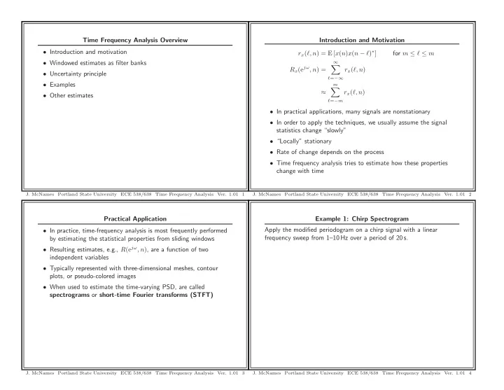
Time Frequency Analysis Overview Introduction and Motivation • Introduction and motivation r x ( ℓ, n ) = E [ x ( n ) x ( n − ℓ ) ∗ ] for m ≤ ℓ ≤ m • Windowed estimates as filter banks ∞ R x (e jω , n ) = � r x ( ℓ, n ) • Uncertainty principle ℓ = −∞ • Examples m � ≈ r x ( ℓ, n ) • Other estimates ℓ = − m • In practical applications, many signals are nonstationary • In order to apply the techniques, we usually assume the signal statistics change “slowly” • “Locally” stationary • Rate of change depends on the process • Time frequency analysis tries to estimate how these properties change with time J. McNames Portland State University ECE 538/638 Time Frequency Analysis Ver. 1.01 1 J. McNames Portland State University ECE 538/638 Time Frequency Analysis Ver. 1.01 2 Practical Application Example 1: Chirp Spectrogram Apply the modified periodogram on a chirp signal with a linear • In practice, time-frequency analysis is most frequently performed frequency sweep from 1–10 Hz over a period of 20 s. by estimating the statistical properties from sliding windows • Resulting estimates, e.g., R (e jω , n ) , are a function of two independent variables • Typically represented with three-dimensional meshes, contour plots, or pseudo-colored images • When used to estimate the time-varying PSD, are called spectrograms or short-time Fourier transforms (STFT) J. McNames Portland State University ECE 538/638 Time Frequency Analysis Ver. 1.01 3 J. McNames Portland State University ECE 538/638 Time Frequency Analysis Ver. 1.01 4

Example 1: Chirp Spectrogram Example 1: Chirp Spectrogram Chirp Signal T w = 0.2 s Chirp Signal T w = 0.5 s 0 2 4 6 8 10 12 14 16 18 20 0 2 4 6 8 10 12 14 16 18 20 10 10 10 10 8 8 8 8 Frequency (Hz) Frequency (Hz) 6 6 6 6 4 4 4 4 2 2 2 2 0 0 0 0 0 2 4 6 8 10 12 14 16 18 20 0 2 4 6 8 10 12 14 16 18 20 Time (s) Time (s) J. McNames Portland State University ECE 538/638 Time Frequency Analysis Ver. 1.01 5 J. McNames Portland State University ECE 538/638 Time Frequency Analysis Ver. 1.01 6 Example 1: Chirp Spectrogram Example 1: Chirp Spectrogram Chirp Signal T w = 2.0 s Chirp Signal T w =15.0 s 0 2 4 6 8 10 12 14 16 18 20 0 2 4 6 8 10 12 14 16 18 20 10 10 10 10 8 8 8 8 Frequency (Hz) Frequency (Hz) 6 6 6 6 4 4 4 4 2 2 2 2 0 0 0 0 0 2 4 6 8 10 12 14 16 18 20 0 2 4 6 8 10 12 14 16 18 20 Time (s) Time (s) J. McNames Portland State University ECE 538/638 Time Frequency Analysis Ver. 1.01 7 J. McNames Portland State University ECE 538/638 Time Frequency Analysis Ver. 1.01 8

Example 1: Relevant MATLAB Code Example 1: Relevant MATLAB Code Continued fs = 20; % Sample rate (Hz) set(gca,’YDir’,’Normal’); T = 20; % Signal duration (s) set(gca,’XAxisLocation’,’Top’); f = [1 10]; % Chirp frequencies [start stop] set(gca,’YAxisLocation’,’Right’); Tw = [0.2 0.5 2 5 15]; % Window lengths xlim([0 T]); ylim([0 fs/2]); k = 0:T*fs; % Discrete time index ht = title(sprintf(’Chirp Signal T_w=%4.1f s’,tw)); t = (k-0.5)/fs; % Sample times (s) ha = axes(’Position’,[0.14 0.10 0.80 0.09]); x = chirp(t,f(1),T,f(2)); h = plot((k-0.5)/fs,x,’b’); set(h,’LineWidth’,0.5); for c1=1:length(Tw), xlim([0 T]); tw = Tw(c1); set(ha,’YTick’,[]) [S,t,f] = NonparametricSpectrogram(x,fs,tw); xlabel(’Time (s)’); figure; I = abs(S).^2; ha = axes(’Position’,[0.07 0.20 0.065 0.73]); cr = prctile(reshape(I,prod(size(I)),1),[0.5 99.5]); Rx = mean(I,2); ha = axes(’Position’,[0.14 0.20 0.80 0.73]); h = plot(Rx,f,’r’); h = imagesc(t,f,abs(S).^2,cr); set(h,’LineWidth’,0.5); hold on; ylim([0 fs/2]); h = plot(tw/2*[1 1],[0 fs/2],’k’,tw/2*[1 1],[0 fs/2],’w’); set(ha,’XTick’,[]) set(h(1),’LineWidth’,2); ylabel(’Frequency (Hz)’); set(h(2),’LineWidth’,1); h = plot((T-tw/2)*[1 1],[0 fs/2],’k’,(T-tw/2)*[1 1],[0 fs/2],’w’); set(ht,’VerticalAlignment’,’Top’) set(h(1),’LineWidth’,2); end; set(h(2),’LineWidth’,1); hold off; J. McNames Portland State University ECE 538/638 Time Frequency Analysis Ver. 1.01 9 J. McNames Portland State University ECE 538/638 Time Frequency Analysis Ver. 1.01 10 Why the Windowed Periodogram? Filter Bank Interpretation • Why not a smoother technique with less variance? ∞ � X (e jω , n ) = x ( n + ℓ ) w ( ℓ )e − jωℓ – The eye can smooth the plots visually ℓ = −∞ – Techniques to decrease variance decrease the resolution too ∞ much � x ( m ) w ( m − n )e − jω ( m − n ) = • Why window the segments? Could use a rectangular window m = −∞ ∞ – If tapered window is not applied, estimate will vary even if the � x ( m ) w ( − ( n − m ))e jω ( n − m ) = signal is a constant sinusoid m = −∞ – Due to variation of phase of sinusoid that is included in the = x ( n ) ∗ w ( − n )e jωn segment (covered by the window) R (MP) (e jω , n ) = 1 ˆ L | X (e jω , n ) | 2 – Taper reduces this effect – Also reduces sidelobe leakage • The spectrogram can be thought of as the squared magnitude of the output of an LTI system with impulse response h ω ( n ) = w ( − n )e jωn � e j ( ω o − ω ) � • The magnitude response evaluated at ω o is then W J. McNames Portland State University ECE 538/638 Time Frequency Analysis Ver. 1.01 11 J. McNames Portland State University ECE 538/638 Time Frequency Analysis Ver. 1.01 12

Filter Bank Frequency Responses without Padding Effect of Zero Padding FFT Filters Blackman Window L=17 P=17 Time Domain Frequency Domain 0.5 3 16 points 12 0 2 10 −0.5 1 −1 0 8 |W(e j ω )| 20 40 60 80 100 120 0 0.1 0.2 0.3 0.4 Frequency Domain 6 128 points (112 zeros) 0.5 3 4 0 2 2 −0.5 1 −1 0 0 0 0.5 1 1.5 2 2.5 3 20 40 60 80 100 120 0 0.1 0.2 0.3 0.4 Frequency (radians/sample) J. McNames Portland State University ECE 538/638 Time Frequency Analysis Ver. 1.01 13 J. McNames Portland State University ECE 538/638 Time Frequency Analysis Ver. 1.01 14 Filter Bank Frequency Responses with Padding Primary Tradeoff: Segment Length • Primary purpose of windowing is to guarantee local stationarity FFT Filters Blackman Window L=17 P=32 • Window shape controls tradeoff between sidelobe leakage and main lob width 12 • Primary parameter is the window length, L 10 • Long window – Poor time resolution 8 |W(e j ω )| – Good frequency resolution – Use with slowly varying signal characteristics 6 • Short window 4 – Good time resolution – Poor frequency resolution 2 – Use with rapidly changing signal characteristics 0 • Thus L primarily controls the tradeoff between time and frequency 0 0.5 1 1.5 2 2.5 3 Frequency (radians/sample) resolution J. McNames Portland State University ECE 538/638 Time Frequency Analysis Ver. 1.01 15 J. McNames Portland State University ECE 538/638 Time Frequency Analysis Ver. 1.01 16

Energy Density Functions Bandwidth • Note that the windowed signal segments have finite energy � ∞ � ∞ µ t,x = t e x ( t ) d t µ ω,x = ω E x ( ω ) d ω • Analogous ideas apply in continuous time −∞ −∞ � ∞ � ∞ • Consider, for a moment, a continuous time windowed segment σ 2 | t − µ t,x | 2 e x ( t ) d t σ 2 | ω − µ ω,x | 2 E x ( ω ) d ω t,x = ω,x = x ( t ) −∞ −∞ • Defined the normalized temporal energy density function and • There are many definitions of duration and bandwidth of a signal spectral energy density function as • One pair of possible definitions is based on the second-order | x ( t ) | 2 | X ( jω ) | 2 moments of the energy density functions e x ( t ) = E x ( ω ) = � ∞ � ∞ −∞ | x ( t ) | 2 d t −∞ | X ( jω ) | 2 d ω • Let us define the signal – Duration as the standard deviation of the temporal edf, σ t,x • Like pdfs, both of these functions are nonnegative and have unit – Bandwidth as the standard deviation of the spectral edf, σ ω,x area • Can be thought of as energy density functions (edfs) in time and frequency • Like pdfs, we can define energy moments J. McNames Portland State University ECE 538/638 Time Frequency Analysis Ver. 1.01 17 J. McNames Portland State University ECE 538/638 Time Frequency Analysis Ver. 1.01 18 Uncertainty Principle Time Bandwidth Product It can be shown that Windowed Sinusoid ω 0 =0.628 rad/sample Frequency Domain σ t,x × σ ω,x ≥ 1 2 1 10 L=33 X(e j ω 0 • In this context, it is not actually an expression of uncertainty 5 −1 – Signals with short duration have broad bandwidth 0 −100 −50 0 50 100 0 1 2 3 – Signals with long duration can have narrow bandwidth 1 20 • Equivalently, if one density is narrow then the other is wide L=65 X(e j ω 0 10 • They can’t both be arbitrarily narrow −1 0 • In quantum mechanics, applies to probability densities of position −100 −50 0 50 100 0 1 2 3 and velocity so uncertainty is appropriate 50 1 L=129 X(e j ω • Not aware of an equivalent uncertainty principle for DT signals 0 −1 0 −100 −50 0 50 100 0 1 2 3 Sample Index (n) Frequency (rad/sec) J. McNames Portland State University ECE 538/638 Time Frequency Analysis Ver. 1.01 19 J. McNames Portland State University ECE 538/638 Time Frequency Analysis Ver. 1.01 20