The role of RiemannHilbert techniques in integrable systems, - PowerPoint PPT Presentation

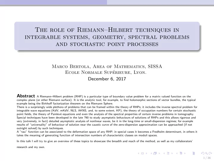
The role of Riemann–Hilbert techniques in integrable systems, geometry, spectral problems and stochastic point processes Marco Bertola, Area of Mathematics, SISSA Ecole Normale Sup´ erieure, Lyon. December 6, 2017 Abstract A Riemann–Hilbert problem (RHP) is a particular type of boundary value problem for a matrix valued function on the complex plane (or other Riemann surface). It is the analytic tool, for example, to find holomorphic sections of vector bundles, the typical example being the Birkhoff factorization theorem on the Riemann Sphere. There is a surprisingly wide plethora of problems that can be framed within the theory of RHPs; it includes the inverse spectral problem for integrable wave equations (KdV, mKdV, NLS, AKNS, and, to some extent, KP), the theory of occupation numbers for certain stochastic point fields, the theory of Painlev´ e equations and even the analysis of the spectral properties of certain inverse problems in tomography. Special techniques have been developed in the late ?90 to study asymptotic behaviours of solutions of RHPs and this allows rigorous and very (extremely, in fact) detailed asymptotic analysis of nonlinear waves, be it in the long-time or small-dispersion regimes; for example results of “universality” of behaviour of solution near the caustic curve of the zero-dispersion approximation can be approached (if not outright solved) by such techniques. A ”tau” function can be associated to the deformation space of any RHP; in special cases it becomes a Fredholm determinant, in others it takes the meaning of generating function of intersection numbers of characteristic classes on moduli spaces. In this talk I will try to give an overview of these topics to showcase the breadth and reach of the method, as well as my collaborators’ research and my own. 1 / 36

We give an overview of the wide range of applications of Riemann–Hilbert problems in recent results. 1 Riemann–Hilbert problems 2 Nonlinear Waves (B. Tovbis ’15, Grava-Claeys ’13, Dubrovin-Grava-Klein ’12) 3 Random (Multi)–Matrices (B.-Gekhtman-Szmigielski ’12, B. Bothner ’15) 4 Spectral properties of tomography (B.-Katsevich-Tovbis, ’15–’17). 5 Intersection numbers (B.-Dubrovin-Di ’16, B.-Cafasso ’16, B.-Ruzza ’17) 6 Integrable systems: Painlev´ e-Calogero-Moser, (Levin-Olshanetsky ’00, Takasaki ’01, B.-Cafasso-Rubtsov ’17) 2 / 36

What is a RHP and why you should care OPs, NLS, KdV, Gap probatilities, Painlev´ e equations, etc. are related to a particular type of boundary value problem in the complex plane. A Riemann–Hilbert problem is a boundary–value problem for a matrix–valued, piecewise analytic function Γ p z q . Problem Let Σ be an oriented (union of) curve(s) and M p z q a (sufficiently smooth) matrix function defined on Σ . Find a matrix-valued function Y p z q with the properties that Y p z q is analytic on C z Σ ; lim z Ñ8 Y p z q “ 1 (or some other normalization); Y ` p z q “ Y ´ p z q M p z q ; @ z P Σ Y ` p z q “ Y ´ p z q M p z q ` ´ 3 / 36

In the scalar case, a RHP is reducible to the Sokhotsky-Plemelji formula Theorem (Sokhotsky-Plemelji formula) Let h p w q be α –H¨ older on Σ and ż 1 h p w q d w e f ` “ e f ´ e h f p z q : “ ñ f ` p w q ´ f ´ p w q “ h p w q ñ (1) 2 iπ w ´ z Σ (Partial) Index problem. In the matrix case the solution cannot be written explicitly (at best an integral equation can be derived) and hence the problem is genuinely transcendental. Can be rephrased as a triviality of a vector bundle (Birkhoff–theorem Ø partial indices) 4 / 36

Tau function Definition (B. ’10, B. ’16) Deformation theory of jump-matrix M p z ; t q leads to ˆ ˙ d z ż Y ´ 1 ´ Y 1 ´ B t MM ´ 1 B t ln τ p t q “ Tr 2 iπ ` Θ p t q (2) Σ Θ is a smooth one form of the deformation parameters (an “anomaly”). First term has a simple pole with integer residue on the Malgrange divisor . The principal property: τ is locally analytic and τ p t q “ 0 if and only if the RHP has no solution (vector bundle is non-trivial). Behaves like a (regularized) Fredholm determinant (Malgrange ’90). Connects with symplectic geometry of the deformation space. Isomonodromic deformations: Painlev´ e and conformal blocks in CFT (Iorgov, Lisovyy, Gamayun, Its, Tykhyy,...’13–onwards) For “oscillatory” problems (depending on parameter), Deift–Zhou method (“non-abelian steepest descent”). 5 / 36

Nonlinear Waves 6 / 36

Nonlinear Schr¨ odinger equation The focusing Nonlinear Schr¨ odinger (NLS) equation, i � B t q “ ´ � 2 B 2 x q ´ 2 | q | 2 q (3) models self-focusing and self-modulation ( optical fibers ). It is integrable by inverse scattering methods (Zakharov–Shabat). It exhibits interesting behaviour as � Ñ 0 ( modulational instability ); in different regions of spacetime, there are different asymptotic behaviors ( phases ) separated by breaking curves (or nonlinear caustics ). 7 / 36

The tip-point of the braking curves is called a point of gradient catastrophe , or elliptic umbilical singularity [Dubrovin-Grava-Klein]. Main goal Leading order asymptotic q p x, t, � q on and around the gradient catastrophe point p x 0 , t 0 q . The behavior in the bulk is described in terms of slow modulation of exact quasi-periodic solutions ( genus 2 ), while outside by slow modulation equations for the amplitude. There are (generically) two types of Umbilical grad catastrophe 4 O p � 5 q transitional regions A strip region of scale O p � ln � q around the breaking curves (nonlinear caustics); O p ǫ ln p ǫ qq 4 5 q around the a circular region of scale O p � O p ǫ q O p ǫ q gradient catastrophe point. Figure: A p x q “ e ´ x 2 , Φ 1p x q “ tanh x and � “ 0 . 03 8 / 36

Zooming in on a peak (B.-Tovbis, ’13) If we scale by � around each peak we find the rational or Peregrine breather ξ “ x ´ x p η “ x ´ x p (4) , � � ˆ ˙ 1 ` 4 ib 2 η Q br p ξ, η q “ e ´ 2 i p aξ `p 2 a 2 ´ b 2 q η q b 1 ´ 4 (5) 1 ` 4 b 2 p ξ ` 4 aη q 2 ` 16 b 4 η 2 i B η Q br ` B 2 ξ Q br ` 2 | Q br | 2 Q br “ 0 (6) 9 / 36

Emergence of “Peregrine breather solution” and time of highest peak after shock predicted analytically in [B.-Tovbis ’13 CPAM] and experimentally verified in nonlinear optics: ”Universality of the Peregrine Soliton in the Focusing Dynamics of the Cubic Nonlinear Schr¨ odinger Equation”, Phys. Rev. Lett. 119 (2017) Tikan-Billet-El-Tovbis-B.-Sylvestre-Gustave-Randoux-Genty-Suret-Dudley 10 / 36

KdV equation and small–dispersion The KdV equation u t “ uu x ` ǫ 2 u xxx , u p x, 0 q “ u 0 p x q rapidly decaying (7) For ǫ “ 0 we have Burger’s equation u t “ uu x , solved by the hodograph method (characteristics), locally f p u q “ u ´ 1 f p u q “ x ` u t (8) 0 1 It shocks at t 0 “ 0 p x q . max u 1 The small-dispersion also exhibits interesting behavior: Near the point of gradient catastrophe p x 0 , t 0 q its behavior is described in terms 6 of a generalization of the Painlev´ e I equation with critical scale � 7 (Dubrovin-Grava-Klein, Grava-Claeys); Near the trailing edge (after the time t 0 ) it is described by the Hastings-McLeod 2 e II equation y 2 p s q “ sy p s q ` 2 y 3 p s q with critical scale � solution of the Painlev´ 3 (Grava-Claeys); Near the leading edge the behavior is described in terms of elementary function (superposition of soliton solutions) with scale � ln � (Grava-Claeys) 11 / 36

KdV-small dispersion KdV-zero dispersion = Burgers 12 / 36

NLS and RHP The nonlinear Schr¨ odinger equation (in 1 spatial dimension) i � q t p x, t q “ ´ � 2 q xx p x, t q ˘ 2 | q p x, t q| 2 q p x, t q (9) Theorem (Zakharov) Let Γ p z ; x, t q be a 2 ˆ 2 matrix, analytic in z P C z R , « ff ´ r p z q e ´ 2 i � p 2 tz 2 ` xz q 1 ´ | r p z q| 2 Γ ` p z ; x, t q “ Γ ´ p z ; x, t q (10) 2 i � p 2 tz 2 ` xz q r p z q e 1 Γ p z ; x, t q “ 1 ` O p z ´ 1 q , | z | Ñ 8 (11) Then the function of x, t q p x, t q : “ 2 i lim z Ñ8 z Γ 12 p z ; x, t q (12) is a solution of the defocusing NLS, with initial data given by the data that was associated to the scattering transform. The advantage of the formulation of the Theorem is that the x, t dependence is in plain sight; the disadvantage is that it is not possible (in general) to obtain a closed formula for the solution of the advocated Riemann–Hilbert problem. 13 / 36

Random Matrices 14 / 36

Random Matrix Models The typical setup: H N : “ t M Hermitean N ˆ N matrix ( M “ M : ) u . d µ : “ d M e ´ tr V p M q (13) ź ź d M “ d ℜ p M ij q d ℑ p M ij q d M kk (14) i ă j k ż Z 1 MM r V s : “ d µ “ Partition function . (15) N B.-Eynard-Harnad (’06) ÿ Z 1 MM t j z j r V s “ τ r V s , V p z q “ N j 15 / 36

The Cauchy chain of positive matrices Definition (The p -chain-Cauchy Matrix-Model, B.-Gekhtman-Szmigielski ’10-13, B.-Bothner ’15) Let M p p q n, ` be the set of p –tuples of positive semidefinite Hermitean matrices with the following class of measures ś p j “ 1 det p M j q a j e ´ N Tr U j p M j q d M j d µ p � M q “ Z (16) ś p ´ 1 j “ 1 det p M j ` M j ` 1 q n The scaling parameter N is taken proportional to the size when considering the limit of large sizes n Ñ 8 . 16 / 36