The resurrection of time as a Time is a covariate determinant of - PDF document
Time The resurrection of time as a Time is a covariate determinant of rates continuous concept in biostatistics, Response variable in survival / follow-up is bivariate: demography and epidemiology Differences on the timescale (
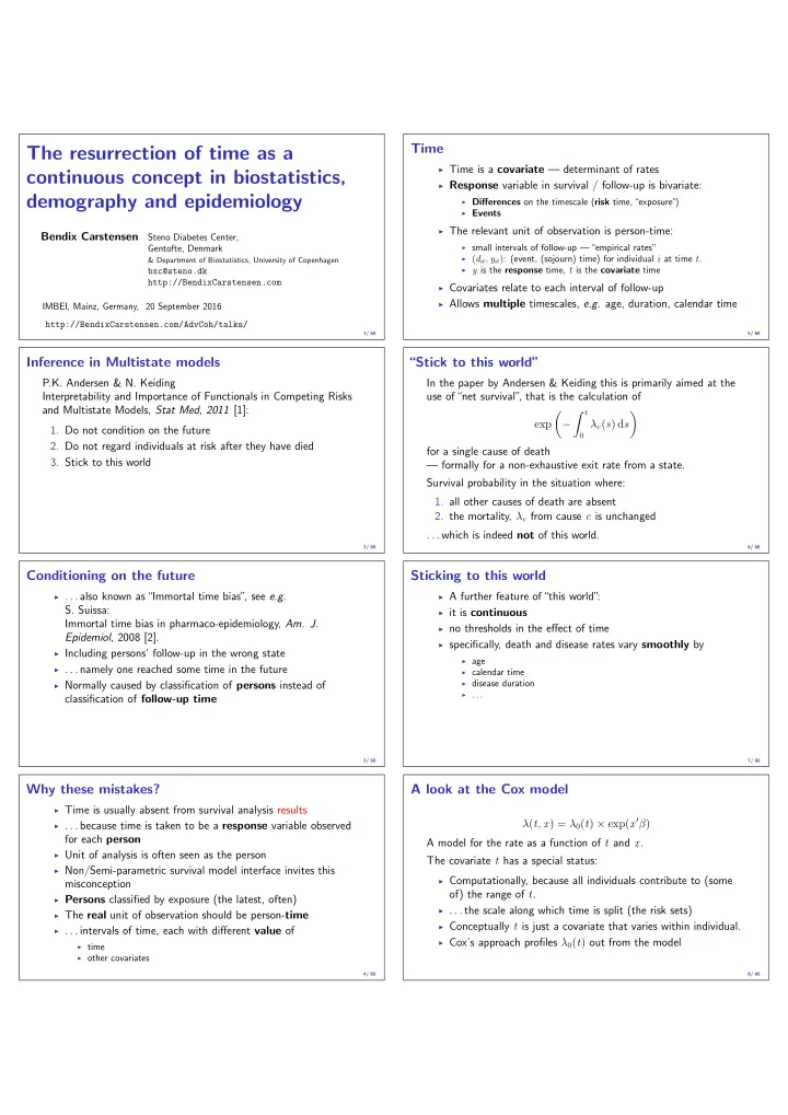
Time The resurrection of time as a ◮ Time is a covariate — determinant of rates continuous concept in biostatistics, ◮ Response variable in survival / follow-up is bivariate: demography and epidemiology ◮ Differences on the timescale ( risk time,“exposure” ) ◮ Events ◮ The relevant unit of observation is person-time: Bendix Carstensen Steno Diabetes Center, ◮ small intervals of follow-up —“empirical rates” Gentofte, Denmark ◮ ( d it , y it ) : (event, (sojourn) time) for individual i at time t . & Department of Biostatistics, University of Copenhagen ◮ y is the response time, t is the covariate time bxc@steno.dk http://BendixCarstensen.com ◮ Covariates relate to each interval of follow-up ◮ Allows multiple timescales, e.g. age, duration, calendar time IMBEI, Mainz, Germany, 20 September 2016 http://BendixCarstensen.com/AdvCoh/talks/ 1/ 60 5/ 60 Inference in Multistate models “Stick to this world” P.K. Andersen & N. Keiding In the paper by Andersen & Keiding this is primarily aimed at the Interpretability and Importance of Functionals in Competing Risks use of“net survival” , that is the calculation of and Multistate Models, Stat Med, 2011 [1]: � t � � exp − λ c ( s ) d s 1. Do not condition on the future 0 2. Do not regard individuals at risk after they have died for a single cause of death 3. Stick to this world — formally for a non-exhaustive exit rate from a state. Survival probability in the situation where: 1. all other causes of death are absent 2. the mortality, λ c from cause c is unchanged . . . which is indeed not of this world. 2/ 60 6/ 60 Conditioning on the future Sticking to this world ◮ . . . also known as“Immortal time bias” , see e.g. ◮ A further feature of“this world” : S. Suissa: ◮ it is continuous Immortal time bias in pharmaco-epidemiology, Am. J. ◮ no thresholds in the effect of time Epidemiol , 2008 [2]. ◮ specifically, death and disease rates vary smoothly by ◮ Including persons’ follow-up in the wrong state ◮ age ◮ . . . namely one reached some time in the future ◮ calendar time ◮ disease duration ◮ Normally caused by classification of persons instead of ◮ . . . classification of follow-up time 3/ 60 7/ 60 Why these mistakes? A look at the Cox model ◮ Time is usually absent from survival analysis results λ ( t , x ) = λ 0 ( t ) × exp( x ′ β ) ◮ . . . because time is taken to be a response variable observed for each person A model for the rate as a function of t and x . ◮ Unit of analysis is often seen as the person The covariate t has a special status: ◮ Non/Semi-parametric survival model interface invites this ◮ Computationally, because all individuals contribute to (some misconception of) the range of t . ◮ Persons classified by exposure (the latest, often) ◮ . . . the scale along which time is split (the risk sets) ◮ The real unit of observation should be person- time ◮ Conceptually t is just a covariate that varies within individual. ◮ . . . intervals of time, each with different value of ◮ Cox’s approach profiles λ 0 ( t ) out from the model ◮ time ◮ other covariates 4/ 60 8/ 60
The Cox-likelihood as profile likelihood The derivative w.r.t. α t is: ◮ One parameter per death time to describe the effect of time 1 e η i = 0 e α t = D α t ℓ t ( α t , β ) = 1 − e α t � ⇔ (i.e. the chosen timescale). � i ∈R t e η i i ∈R t � � � � log λ ( t , x i ) = log λ 0 ( t ) + β 1 x 1 i + · · · + β p x pi = α t + η i If this estimate is fed back into the log-likelihood for α t , we get the profile likelihood (with α t “profiled out” ): ◮ Profile likelihood: ◮ Derive estimates of α t as function of data and β s � � � e η death � 1 — assuming constant rate between death times log + η death − 1 = log − 1 ◮ Insert in likelihood, now only a function of data and β s � i ∈R t e η i � i ∈R t e η i ◮ Turns out to be Cox’s partial likelihood which is the same as the contribution from time t to Cox’s partial likelihood. 9/ 60 13/ 60 The Cox-likelihood: mechanics of computing Splitting the dataset a priori ◮ The likelihood is computed by suming over risk-sets: ◮ The Poisson approach needs a dataset of empirical rates ( d , y ) with suitably small values of y . � e η death � ◮ — each individual contributes many empirical rates � ℓ ( η ) = log � i ∈R t e η i ◮ (one per risk-set contribution in Cox-modelling) t ◮ From each empirical rate we get: ◮ this is essentially splitting follow-up time at event- (and ◮ Poisson-response d ◮ Risk time y → log( y ) as offset censoring) times ◮ Covariate value for the timescale ◮ . . . repeatedly in every cycle of the iteration (time since entry, current age, current date, . . . ) ◮ . . . simplified by not keeping track of risk time ◮ other covariates ◮ Contributions not independent, but likelihood is a product ◮ . . . but only works along one time scale ◮ Same likelihood as for independent Poisson variates ◮ Modelling is by standard glm Poisson 10/ 60 14/ 60 Example: Mayo Clinic lung cancer � � � � log λ ( t , x i ) = log λ 0 ( t ) + β 1 x 1 i + · · · + β p x pi = α t + η i ◮ Survival after lung cancer ◮ Covariates: ◮ Suppose the time scale has been divided into small intervals ◮ Age at diagnosis with at most one death in each: ◮ Sex ◮ Empirical rates: ( d it , y it ) — each t has at most one d it = 0 . ◮ Time since diagnosis ◮ Assume w.l.o.g. the y s in the empirical rates all are 1. ◮ Cox model ◮ Log-likelihood contributions that contain information on a ◮ Split data: specific time-scale parameter α t will be from: ◮ Poisson model, time as factor ◮ Poisson model, time as spline ◮ the (only) empirical rate (1 , 1) with the death at time t . ◮ all other empirical rates (0 , 1) from those who were at risk at time t . 11/ 60 15/ 60 Note: There is one contribution from each person at risk to this Mayo Clinic 1.0 part of the log-likelihood: lung cancer 0.8 60 year old woman � ℓ t ( α t , β ) = d i log( λ i ( t )) − λ i ( t ) y i i ∈R t 0.6 � d i ( α t + η i ) − e α t + η i � � Survival = i ∈R t 0.4 = α t + η death − e α t � e η i i ∈R t 0.2 where η death is the linear predictor for the person that died. 0.0 0 200 400 600 800 Days since diagnosis 12/ 60 16/ 60
Recommend
More recommend
Explore More Topics
Stay informed with curated content and fresh updates.

