The response of wall turbulence to streamwise-traveling waves of - PowerPoint PPT Presentation
Background The traveling waves Results Interpretation The response of wall turbulence to streamwise-traveling waves of spanwise wall velocity M.Quadrio Politecnico di Milano maurizio.quadrio@polimi.it iTi 2008, Bertinoro, Oct 12-15
Background The traveling waves Results Interpretation The response of wall turbulence to streamwise-traveling waves of spanwise wall velocity M.Quadrio Politecnico di Milano maurizio.quadrio@polimi.it iTi 2008, Bertinoro, Oct 12-15
Background The traveling waves Results Interpretation Outline Background 1 The traveling waves 2 Results 3 Interpretation 4
Background The traveling waves Results Interpretation Outline Background 1 The traveling waves 2 Results 3 Interpretation 4
Background The traveling waves Results Interpretation Spanwise wall forcing of turbulence A long story made short 1985 Bradshaw & Pontikos 1985: sudden spanwise pressure gradient 1992 Jung et al. 1992: harmonic spanwise wall oscillation 1993- many papers on the oscillating-wall technique
Background The traveling waves Results Interpretation Spanwise wall oscillation: the essentials w ( x , y = 0 , z , t ) = A sin ( ω t ) High levels of turbulent friction drag reduction Basic mechanism still elusive Existence of an optimum period T opt Unpractical because of moving parts
Background The traveling waves Results Interpretation An important concept: the convection velocity Turbulent fluctuations at the wall possess a convection velocity Known concept (Kreplin & Eckelmann) in the ’70 Re-discovered (!) by Kim & Hussain ’93 Re-re-discovered (!!) by Quadrio & Luchini ’03
Background The traveling waves Results Interpretation The oscillating wall made stationary w ( x , y = 0 , z , t ) = A sin ( κ x ) Convection allows translating the oscillation into a steady forcing Existence of an optimal wavelength λ opt = U w T opt Easily implemented as a passive device (sinusoidal riblets, other roughness)
Background The traveling waves Results Interpretation Outline Background 1 The traveling waves 2 Results 3 Interpretation 4
Background The traveling waves Results Interpretation The traveling waves: an obvious curiosity w = A sin ( ω t ) w = A sin ( κ x ) w = A sin ( κ x − ω t ) Oscillating wall Steady waves Traveling waves Phase speed Infinite phase Zero phase speed speed c = ω / κ
Background The traveling waves Results Interpretation A numerical DNS study DNS pseudo-spectral code Parallel strategy to exploit commodity hardware (Luchini & Quadrio JCP 2006) Powerful dedicated system with 268 dual-core Opteron CPUs, 280GB RAM, 40TB disk space
Background The traveling waves Results Interpretation A large parametric study Turbulent channel flow at Re τ = 200 Standard domain size: L x = 6 π h , L y = 2 h and L z = 3 π h Standard spatial resolution: N x = 320, N y = 160 and N z = 320 Long averaging time More than 250 simulations Approx. 4 centuries of CPU time
Background The traveling waves Results Interpretation Outline Background 1 The traveling waves 2 Results 3 Interpretation 4
Background The traveling waves Results Interpretation Unexpected results! Waves may yield both DR and DI
Background The traveling waves Results Interpretation How much power to generate the waves? Power ∼ w ∂ w / ∂ y | y = 0 Upper bound to energetic cost Similar to drag reduction map! Ratio of energy save to cost up to 30:1 Up to 25% net energy save
Background The traveling waves Results Interpretation Outline Background 1 The traveling waves 2 Results 3 Interpretation 4
Background The traveling waves Results Interpretation Understanding the physics The lifetime T ℓ of turbulent structures
Background The traveling waves Results Interpretation Unsteadiness in the convecting reference frame Oscillating wall Forcing on a timescale ≫ T ℓ does not yield DR Timescale: oscillation period T
Background The traveling waves Results Interpretation Unsteadiness in the convecting reference frame Oscillating wall Traveling waves Forcing on a timescale Forcing on a timescale ≫ T ℓ does not yield DR ≫ T ℓ does not yield DR Timescale: oscillation Timescale: oscillation period T period T as seen in a convecting reference frame λ x T = U w − c U w : convection velocity at the wall c = ω / κ : phase speed
Background The traveling waves Results Interpretation How spanwise forcing really works (1)
Background The traveling waves Results Interpretation One step back Extending the laminar Stokes solution w ( y , t ) Laminar case Transverse, w ( y , x ) alternating boundary layer Qualitative similarity w ( y , x − ct )
Background The traveling waves Results Interpretation The generalized Stokes layer An analytical approximate solution � � � 1 / 3 � ��� � 2 π u y , 0 y − c Ce 2 π i ( x − ct ) / λ x Ai e π i / 6 w ( x , y , t ) = A ℜ λ x ν u y , 0 δ GSL ≪ h Neglect streamwise viscous diffusion Threshold velocity to discriminate flow regimes
Background The traveling waves Results Interpretation Using the GLS solution Thickness of the GLS
Background The traveling waves Results Interpretation How spanwise forcing really works (2)
Background The traveling waves Results Interpretation Future work Understanding scaling properties of DR (laminar solution available!) Really understanding how spanwise forcing really works Real device?
Recommend
More recommend
Explore More Topics
Stay informed with curated content and fresh updates.
