The Power of Low-Degree Polynomials for Solving Statistical Problems - PowerPoint PPT Presentation

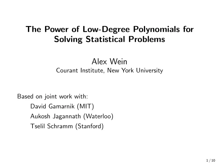
The Power of Low-Degree Polynomials for Solving Statistical Problems Alex Wein Courant Institute, New York University Based on joint work with: David Gamarnik (MIT) Aukosh Jagannath (Waterloo) Tselil Schramm (Stanford) 1 / 10

Problems in High-Dimensional Statistics Example: finding a large clique in a random graph 2 / 10

Problems in High-Dimensional Statistics Example: finding a large clique in a random graph ◮ Detection : distinguish between a random graph and a graph with a planted clique 2 / 10

Problems in High-Dimensional Statistics Example: finding a large clique in a random graph ◮ Detection : distinguish between a random graph and a graph with a planted clique ◮ Recovery : given a graph with a planted clique, find the clique 2 / 10

Problems in High-Dimensional Statistics Example: finding a large clique in a random graph ◮ Detection : distinguish between a random graph and a graph with a planted clique ◮ Recovery : given a graph with a planted clique, find the clique ◮ Optimization : given a random graph (with no planted clique), find as large a clique as possible 2 / 10

Problems in High-Dimensional Statistics Example: finding a large clique in a random graph ◮ Detection : distinguish between a random graph and a graph with a planted clique ◮ Recovery : given a graph with a planted clique, find the clique ◮ Optimization : given a random graph (with no planted clique), find as large a clique as possible Common to have information-computation gaps 2 / 10

Problems in High-Dimensional Statistics Example: finding a large clique in a random graph ◮ Detection : distinguish between a random graph and a graph with a planted clique ◮ Recovery : given a graph with a planted clique, find the clique ◮ Optimization : given a random graph (with no planted clique), find as large a clique as possible Common to have information-computation gaps E.g. planted k -clique (either detection or recovery) 2 / 10

Problems in High-Dimensional Statistics Example: finding a large clique in a random graph ◮ Detection : distinguish between a random graph and a graph with a planted clique ◮ Recovery : given a graph with a planted clique, find the clique ◮ Optimization : given a random graph (with no planted clique), find as large a clique as possible Common to have information-computation gaps E.g. planted k -clique (either detection or recovery) What makes problems easy vs hard? 2 / 10

The Low-Degree Polynomial Method A framework for understanding computational complexity 3 / 10

The Low-Degree Polynomial Method A framework for understanding computational complexity Originated from sum-of-squares literature (for detection) [Barak, Hopkins, Kelner, Kothari, Moitra, Potechin ’16] [Hopkins, Steurer ’17] [Hopkins, Kothari, Potechin, Raghavendra, Schramm, Steurer ’17] [Hopkins ’18 (PhD thesis)] 3 / 10

The Low-Degree Polynomial Method A framework for understanding computational complexity Originated from sum-of-squares literature (for detection) Study a restricted class of algorithms: low-degree polynomials 3 / 10

The Low-Degree Polynomial Method A framework for understanding computational complexity Originated from sum-of-squares literature (for detection) Study a restricted class of algorithms: low-degree polynomials ◮ Multivariate polynomial f : R N → R M 3 / 10

The Low-Degree Polynomial Method A framework for understanding computational complexity Originated from sum-of-squares literature (for detection) Study a restricted class of algorithms: low-degree polynomials ◮ Multivariate polynomial f : R N → R M ◮ “Low” means O (log n ) where n is dimension 3 / 10

The Low-Degree Polynomial Method A framework for understanding computational complexity Originated from sum-of-squares literature (for detection) Study a restricted class of algorithms: low-degree polynomials ◮ Multivariate polynomial f : R N → R M ◮ “Low” means O (log n ) where n is dimension Some low-degree algorithms: 3 / 10

The Low-Degree Polynomial Method A framework for understanding computational complexity Originated from sum-of-squares literature (for detection) Study a restricted class of algorithms: low-degree polynomials ◮ Multivariate polynomial f : R N → R M ◮ “Low” means O (log n ) where n is dimension Some low-degree algorithms: ◮ Spectral methods (power iteration) 3 / 10

The Low-Degree Polynomial Method A framework for understanding computational complexity Originated from sum-of-squares literature (for detection) Study a restricted class of algorithms: low-degree polynomials ◮ Multivariate polynomial f : R N → R M ◮ “Low” means O (log n ) where n is dimension Some low-degree algorithms: ◮ Spectral methods (power iteration) ◮ Approximate message passing (AMP) [DMM09] 3 / 10

The Low-Degree Polynomial Method A framework for understanding computational complexity Originated from sum-of-squares literature (for detection) Study a restricted class of algorithms: low-degree polynomials ◮ Multivariate polynomial f : R N → R M ◮ “Low” means O (log n ) where n is dimension Some low-degree algorithms: ◮ Spectral methods (power iteration) ◮ Approximate message passing (AMP) [DMM09] Low-degree algorithms are as powerful as the best known polynomial-time algorithms for many problems : planted clique, sparse PCA, community detection, tensor PCA, constraint satisfaction, spiked matrix [BHKKMP16,HS17,HKPRSS17,Hop18,BKW19,KWB19,DKWB19] 3 / 10

Overview This talk: techniques to prove that all low-degree polynomials fail 4 / 10

Overview This talk: techniques to prove that all low-degree polynomials fail Constitutes evidence for computational hardness 4 / 10

Overview This talk: techniques to prove that all low-degree polynomials fail Constitutes evidence for computational hardness Settings: ◮ Detection (prior work) ◮ Recovery Schramm, W. “Computational Barriers to Estimation from Low-Degree Polynomials”, arXiv, 2020. ◮ Optimization Gamarnik, Jagannath, W. “Low-Degree Hardness of Random Optimization Problems”, FOCS 2020. 4 / 10

Detection (e.g. [Hopkins, Steurer ’17] ) Goal: hypothesis test with error probability o (1) between: ◮ Null model Y ∼ Q n e.g. G ( n , 1 / 2) ◮ Planted model Y ∼ P n e.g. G ( n , 1 / 2) ∪ { random k -clique } 5 / 10

Detection (e.g. [Hopkins, Steurer ’17] ) Goal: hypothesis test with error probability o (1) between: ◮ Null model Y ∼ Q n e.g. G ( n , 1 / 2) ◮ Planted model Y ∼ P n e.g. G ( n , 1 / 2) ∪ { random k -clique } Look for a degree- D (multivariate) polynomial f : R n × n → R that distinguishes P from Q 5 / 10

Detection (e.g. [Hopkins, Steurer ’17] ) Goal: hypothesis test with error probability o (1) between: ◮ Null model Y ∼ Q n e.g. G ( n , 1 / 2) ◮ Planted model Y ∼ P n e.g. G ( n , 1 / 2) ∪ { random k -clique } Look for a degree- D (multivariate) polynomial f : R n × n → R that distinguishes P from Q ◮ In the sense that f ( Y ) is “big” when Y ∼ P and “small” when Y ∼ Q 5 / 10

Detection (e.g. [Hopkins, Steurer ’17] ) Goal: hypothesis test with error probability o (1) between: ◮ Null model Y ∼ Q n e.g. G ( n , 1 / 2) ◮ Planted model Y ∼ P n e.g. G ( n , 1 / 2) ∪ { random k -clique } Look for a degree- D (multivariate) polynomial f : R n × n → R that distinguishes P from Q ◮ In the sense that f ( Y ) is “big” when Y ∼ P and “small” when Y ∼ Q E Y ∼ P [ f ( Y )] mean in P Compute max � fluctuations in Q E Y ∼ Q [ f ( Y ) 2 ] f deg D 5 / 10

Detection (e.g. [Hopkins, Steurer ’17] ) Goal: hypothesis test with error probability o (1) between: ◮ Null model Y ∼ Q n e.g. G ( n , 1 / 2) ◮ Planted model Y ∼ P n e.g. G ( n , 1 / 2) ∪ { random k -clique } Look for a degree- D (multivariate) polynomial f : R n × n → R that distinguishes P from Q ◮ In the sense that f ( Y ) is “big” when Y ∼ P and “small” when Y ∼ Q E Y ∼ P [ f ( Y )] mean in P Compute max � fluctuations in Q E Y ∼ Q [ f ( Y ) 2 ] f deg D � ω (1) degree- D polynomial succeed = O (1) degree- D polynomials fail 5 / 10

Detection (e.g. [Hopkins, Steurer ’17] ) E Y ∼ P [ f ( Y )] max � E Y ∼ Q [ f ( Y ) 2 ] f deg D 6 / 10

Detection (e.g. [Hopkins, Steurer ’17] ) E Y ∼ P [ f ( Y )] max � f , g � = E Y ∼ Q [ f ( Y ) g ( Y )] � E Y ∼ Q [ f ( Y ) 2 ] f deg D � � f � = � f , f � 6 / 10

Detection (e.g. [Hopkins, Steurer ’17] ) E Y ∼ P [ f ( Y )] max � f , g � = E Y ∼ Q [ f ( Y ) g ( Y )] � E Y ∼ Q [ f ( Y ) 2 ] f deg D � E Y ∼ Q [ L ( Y ) f ( Y )] � f � = � f , f � = max � E Y ∼ Q [ f ( Y ) 2 ] f deg D Likelihood ratio: L ( Y ) = d P d Q ( Y ) 6 / 10

Detection (e.g. [Hopkins, Steurer ’17] ) E Y ∼ P [ f ( Y )] max � f , g � = E Y ∼ Q [ f ( Y ) g ( Y )] � E Y ∼ Q [ f ( Y ) 2 ] f deg D � E Y ∼ Q [ L ( Y ) f ( Y )] � f � = � f , f � = max � E Y ∼ Q [ f ( Y ) 2 ] f deg D � L , f � Likelihood ratio: = max L ( Y ) = d P � f � d Q ( Y ) f deg D 6 / 10