The Poisson Distribution August 15, 2019 August 15, 2019 1 / 26 - PowerPoint PPT Presentation
The Poisson Distribution August 15, 2019 August 15, 2019 1 / 26 Midterm Results Statistic Raw Score Percentage Mean 32.2 71.5 Median 32 71.1 Standard Deviation 5.0 10.8 Maximum 42 93.3 Minimum 19 42.2 Note: Raw scores are out
The Poisson Distribution August 15, 2019 August 15, 2019 1 / 26
Midterm Results Statistic Raw Score Percentage Mean 32.2 71.5 Median 32 71.1 Standard Deviation 5.0 10.8 Maximum 42 93.3 Minimum 19 42.2 Note: Raw scores are out of 45 possible points. Any extra credit has already been added to the midterm scores. Midterm Results August 15, 2019 2 / 26
Calculating Your Current Grade You can use a little bit of statistics to calculate your current grade! Labs are worth 10% Quizzes (homeworks) are work 20% The midterm is worth 30% The final will be worth 40% Midterm Results August 15, 2019 3 / 26
Calculating Your Current Grade You have grades for 10% + 20% = 30% = 60% of the class. We can use this to scale these values and calculate your current overall grade. For your current grade, labs are worth 0 . 1 / 0 . 6 = 0 . 1667 or 16.67% Quizzes (homeworks) are worth . 2 /. 6 = 0 . 3333 or 33.33% And the midterm is worth . 3 /. 6 = 0 . 50 or 50% Midterm Results August 15, 2019 4 / 26
Calculating Your Current Grade We can use these to calculate a weighted average. This will give you your current grade. 0 . 167 × (Lab %) + 0 . 333 × (Quiz %) + 0 . 5 × (Midterm %) This is just like calculating an expected value! Midterm Results August 15, 2019 5 / 26
Calculating Your Current Grade So if I have 100% in lab, an 85% on quizzes, and got a 70% on the midterm, my current grade is 0 . 167 × (1) + 0 . 333 × (0 . 85) + 0 . 5 × (0 . 7) = 0 . 80 Note: Remember we drop your lowest lab score! There is also still time to get your quiz grade up a bit. Midterm Results August 15, 2019 6 / 26
Midterm Results The labs and quizzes are designed to help pad your grade. If you’re showing up to lab and doing well on your quizzes, I am not worried about your ability to excel in this course. If you calculate your grade and it’s lower than you want it to be, let’s talk! If overall grades at the end of the term are low, I will ”curve” the class by adding a set number of points to everyone’s grade . Midterm Results August 15, 2019 7 / 26
Working With Cumulative Probabilities Practice rewriting the following probabilities in terms of P ( X ≤ x ) and P ( X = x 1 ) + P ( X = x 2 ) + . . . . P ( X < 4) P ( X > 4) P ( X ≤ 4) P ( X ≥ 4) Section 4.5 August 15, 2019 8 / 26
Working With Cumulative Probabilities Practice rewriting the following probabilities in terms of P ( X ≤ x ) and P ( X = x 1 ) + P ( X = x 2 ) + . . . . P (6 ≤ X ≤ 8) P (6 ≤ X < 8) P (6 < X ≤ 8) P (6 < X < 8) Section 4.5 August 15, 2019 9 / 26
Motivating Example: Poisson Distribution There are about 8 million people in New York City. How many New Yorkers would be expect to be hospitalized due to heat attack, each day? Historical records suggest the average is 4.4 But what about the distribution? What might a histogram of daily counts look like? Section 4.5 August 15, 2019 10 / 26
Example Intuitively, we might think that The average is 4.4. We don’t know the standard deviation. The minimum is 0. The (theoretical) maximum is about 800 million or so. It’s so far away from the mean as to be meaningless. Clearly the maximum is a lot further from the average than the minimum is, so we might guess that this distribution is skewed to the right. Section 4.5 August 15, 2019 11 / 26
Example The number of heart attack hospitalizations were recorded every day for a year. The sample mean is 4.38, similar to the historical average of 4.4. The sample standard deviation is about 2. The distribution is unimodal and right-skewed. Section 4.5 August 15, 2019 12 / 26
The Poisson Distribution The Poisson distribution is used to describe the number of events that occur in a large population over some period of time. We might measure Marriages Births Heart attacks Lightning strikes In each case, we can count the number of times that event occurs during a period of time. Section 4.5 August 15, 2019 13 / 26
The Poisson Distribution The average number of occurrences per period of time is called the rate . In the heart attack example, we had a rate of 4.4 heart attacks (the event) per day (the period of time). We denote the rate by the Greek letters λ (lambda) or µ . We can use this information to find the probability of observing exactly k events during a particular period of time. Section 4.5 August 15, 2019 14 / 26
The Poisson Distribution Suppose we are interested in some events and the number of observed events follows a Poisson distribution with rate λ . Let X be the number of events observed. Then P ( X = k ) = λ k e − λ . k ! where k can take on any whole number greater than or equal to 0. The letter e is a constant: e ≈ 2 . 719. Section 4.5 August 15, 2019 15 / 26
The Poisson Distribution The Poisson distribution has an interesting property: its mean and variance are the same! E ( X ) = V ar ( X ) = λ √ and the standard deviation is then λ . Section 4.5 August 15, 2019 16 / 26
Is It Poisson? Guidelines for determining if the Poisson distribution is appropriate: 1 We are interested in the number of events that occur. 2 There is a set period of time that we are interested in. 3 Events occur independently of each other. 4 The population that generates the events is quite large. Section 4.5 August 15, 2019 17 / 26
Example: Coffee Shop Customers A coffee shop serves an average of 75 customers per hour during the morning rush. Which distribution is appropriate for working with the probability of a given number of customers arriving within one hour during the morning rush? Section 4.5 August 15, 2019 18 / 26
Example: Coffee Shop Customers 1 We are interested in the number of customers served. ”Customer served” is the event. 2 We are interested in this event over the course of one hour (during morning rush), so there is a set period of time. 3 We assume that customers are served (more or less) independently of one another. 4 The population that generates these events is anyone who could possibly walk in and be served during the morning rush. That’s quite a lot of people, so can be confident that the population is large. So the Poisson distribution is appropriate. Section 4.5 August 15, 2019 19 / 26
Example: Coffee Shop Customers What are the mean and standard deviation of the number of customers this coffee shop serves in one hour during the morning rush? Section 4.5 August 15, 2019 20 / 26
Example: Coffee Shop Customers Would it be considered unusually low if only 60 customers showed up to the coffee shop in one hour during the morning rush? Section 4.5 August 15, 2019 21 / 26
Example: Coffee Shop Customers Find the probability that the coffee shop serves 70 people in one hour during the morning rush. Section 4.5 August 15, 2019 22 / 26
Example: Coffee Shop Customers What is the probability that the coffee shop serves between (and including) 73 and 76 customers? Section 4.5 August 15, 2019 23 / 26
Poisson Approximation to Binomial This is another binomial approximation method that will help us avoid difficult factorial expressions. We can use the Poisson approximation to the binomial distribution when n is large np < 7 Section 4.5 August 15, 2019 24 / 26
Poisson Approximation to Binomial Suppose we have a lot size of 1000 and the proportion of defective items is 0.001. What is the probability of exactly 3 defective items? Items are either defective or not. Defective status is independent between items. There is a fixed lot size of n = 1000 items. The probability of success (a defect) is 0.001. Section 4.5 August 15, 2019 25 / 26
The binomial probability for exactly 3 defectives is � 1000 � (0 . 001) 3 (0 . 999) 1000 − 3 P ( X = 3) = 3 = 0 . 0613 OR, we can let λ = np = 1 and use the Poisson distribution: P ( X = 3) = e − 1 1 3 3! = 0 . 0613 Section 4.5 August 15, 2019 26 / 26
Recommend
More recommend
Explore More Topics
Stay informed with curated content and fresh updates.

