the law of large numbers & the CLT 0.020 n = 4 0.015 - PowerPoint PPT Presentation

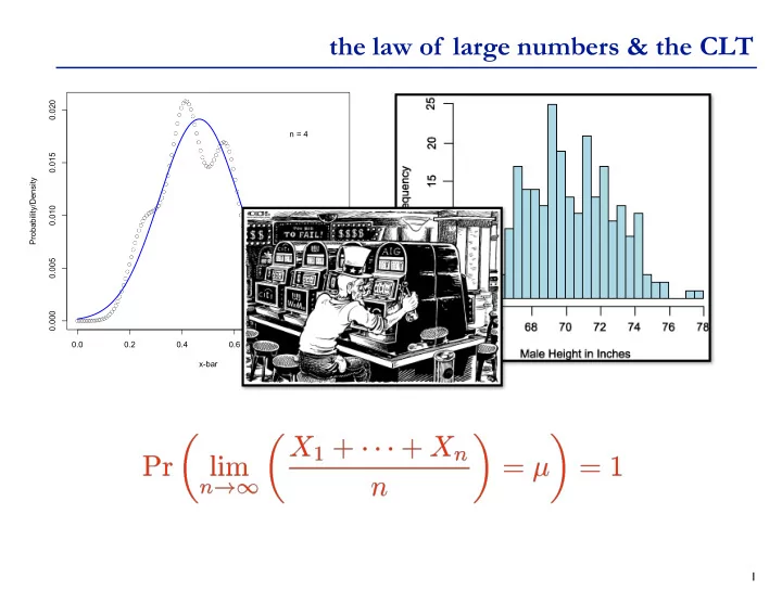
the law of large numbers & the CLT 0.020 n = 4 0.015 Probability/Density 0.010 0.005 0.000 0.0 0.2 0.4 0.6 0.8 1.0 x-bar 1

sums of random variables If X,Y are independent, what is the distribution of Z = X + Y ? Discrete case: p Z ( z ) = Σ x p X ( x ) • p Y ( z-x ) y = z - x Continuous case: + ∞ f Z ( z ) = ∫ f X ( x ) • f Y ( z-x ) dx - ∞ E.g. what is the p.d.f. of the sum of 2 normal RV’s? W = X + Y + Z ? Similar, but double sums/integrals V = W + X + Y + Z ? Similar, but triple sums/integrals 2

example If X and Y are uniform , then Z = X + Y is not ; it’s triangular (like dice) : 0.045 0.030 n = 2 0.040 0.025 Probability/Density Probability/Density 0.035 0.020 0.015 0.030 n = 1 0.010 0.025 0.005 0.020 0.000 0.0 0.2 0.4 0.6 0.8 1.0 0.0 0.2 0.4 0.6 0.8 1.0 x-bar x-bar Y ≈ 0 or ≈ 1 is rare, but many ways to get X + Y ≈ 0.5 Intuition: X + 3

moment generating functions aka transforms; b&t 229 Powerful math tricks for dealing with distributions We won’t do much with it, but mentioned/used in book, so a very brief introduction: The k th moment of r.v. X is E[X k ] ; M.G.F. is M(t) = E[e tX ] Closely related to Laplace transforms, which you may have seen. 4

mgf examples An example: MGF of normal( μ , σ 2 ) is exp( μ t+ σ 2 t 2 /2) Two key properties: 1. MGF of sum independent r.v.s is product of MGFs: M X+Y (t) = E[e t(X+Y) ] = E[e tX e tY ] = E[e tX ] E[e tY ] = M X (t) M Y (t) 2. Invertibility: MGF uniquely determines the distribution. e.g.: M X (t) = exp(at+bt 2 ), with b>0, then X ~ Normal(a,2b) Important example: sum of independent normals is normal: X~Normal( μ 1 , σ 1 2 ) Y~Normal( μ 2 , σ 2 2 ) M X+Y (t) = exp( μ 1 t + σ 12 t 2 /2) • exp( μ 2 t + σ 22 t 2 /2) = exp[( μ 1 + μ 2 )t + ( σ 12 + σ 22 )t 2 /2] So X+Y has mean ( μ 1 + μ 2 ), variance ( σ 12 + σ 22 ) (duh) and is normal! 
 ( way easier than slide 2 way!) 5


 
 
 
 “laws of large numbers” Consider i.i.d. (independent, identically distributed) R.V.s 
 X 1 , X 2 , X 3 , … Suppose X i has μ = E[X i ] < ∞ and σ 2 = Var[X i ] < ∞ . 
 What are the mean & variance of their sum? So limit as n →∞ does not exist (except in the degenerate case where μ = 0; note that if μ = 0, the center of the data stays fixed, but if σ 2 > 0, then the variance is unbounded, i.e., its spread grows with n). 6

weak law of large numbers Consider i.i.d. (independent, identically distributed) R.V.s X 1 , X 2 , X 3 , … Suppose X i has μ = E[X i ] < ∞ and σ 2 = Var[X i ] < ∞ n M n = 1 What about the sample mean , as n →∞ ? X X i n i =1  X 1 + · · · + X n � E [ M n ] = E = µ n = σ 2  X 1 + · · · + X n � Var [ M n ] = Var n n So, limits do exist; mean is independent of n, variance shrinks. 7

weak law of large numbers n Continuing: iid RVs X 1 , X 2 , X 3 , …; μ = E[X i ]; σ 2 = M n = 1 Var[X i ]; X X i n i =1 = σ 2  X 1 + · · · + X n � Var [ M n ] = Var n n Expectation is an important guarantee. BUT : observed values may be far from expected values. E.g., if X i ~ Bernoulli( ½ ), the E[ X i ]= ½ , but X i is NEVER ½ . Is it also possible that sample mean of X i ’ s will be far from ½ ? Always? Usually? Sometimes? Never? 8

weak law of large numbers b&t 5.2 For any ε > 0, as n → ∞ Pr ( | M n − µ | > ✏ ) → 0 Proof: ( assume σ 2 < ∞ ; theorem true without that, but harder proof )  X 1 + · · · + X n � E [ M n ] = E = µ n = σ 2  X 1 + · · · + X n � Var [ M n ] = Var n n By Chebyshev inequality, Pr ( | M n − µ | > ✏ ) ≤ � 2 n →∞ > 0 n ✏ 2 9

strong law of large numbers b&t 5.5 i.i.d. (independent, identically distributed) random vars n M n = 1 X 1 , X 2 , X 3 , … X X i n i =1 X i has μ = E[X i ] < ∞ Strong Law ⇒ Weak Law (but not vice versa) Strong law implies that for any ε > 0, there are only a finite number of n satisfying the weak law condition 
 | M n − µ | ≥ ✏ (almost surely, i.e., with probability 1) Supports the intuition of probability as long term frequency 10

weak vs strong laws Weak Law: Strong Law: How do they differ? Imagine an infinite 2-D table, whose rows are indp infinite sample sequences X i . Pick ε . Imagine cell m,n lights up if average of 1 st n samples in row m is > ε away from μ . WLLN says fraction of lights in n th column goes to zero as n →∞ . It does not prohibit every row from having ∞ lights, so long as frequency declines. SLLN also says only a vanishingly small fraction of rows can have ∞ lights. 11

weak vs strong laws – supplement The differences between the WLLN & SLLN are subtle, and not critically important for this course, but for students wanting to know more (e.g., not on exams) , here is my summary. Both “laws” rigorously connect long-term averages of repeated, independent observations to mathematical expectation, justifying the intuitive motivation for E[.]. Specifically, both say that the sequence of (non-i.i.d.) rvs derived from any sequence of M n = P n i =1 X i /n i.i.d. rvs X i converge to E[ X i ]= μ . The strong law totally subsumes the weak law, but the later remains interesting because (a) of its simple proof (Khintchine, early 20th century; using Cheybeshev’s inequality (1867)) and (b) historically (WLLN was proved by Bernoulli ~1705, for Bernoulli rvs, >150 years before Chebyshev [Ross, p391]). The technical difference between WLLN and SLLN is in the definition of convergence. Definition: Let Y i be any sequence of rvs (i.i.d. not assumed) and c a constant. 
 Y i converges to c in probability if ∀ ✏ > 0 , lim n →∞ Pr ( | Y n − c | > ✏ ) = 0 Y i converges to c with probability 1 if Pr (lim n →∞ Y n = c ) = 1 The weak law is the statement that M n converges in probability to μ ; the strong law states it converges with probability 1 to μ . The strong law subsumes the weak law since convergence with probability 1 implies convergence in probability for any sequence Y i of rvs (B&T problem 5.5-15). B&T ex 5.15 illustrates the failure of the converse. A second counterexample is given on the following slide. 12

weak vs strong laws – supplement Example: Consider the sequence of rvs Y n ~ Ber(1/n) Recall the definition of convergence in probability: ∀ ✏ > 0 , lim n →∞ Pr ( | Y n − c | > ✏ ) = 0 Then Y n converges to c = 0 in probability since Pr( Y n > ε ) = 1/n for any 0 < ε <1, hence the limit as n →∞ is 0, satisfying the definition. Recall that Y n converges to c with probability 1 if Pr (lim n →∞ Y n = c ) = 1 However, I claim that does not exist, hence doesn’t equal zero with Pr (lim n →∞ Y n = probability 1. Why no limit? A 0/1 sequence will have a limit if and only if it is all 0 after some finite point (i.e., contains only a finite number of 1’s) or vice versa. But the expected number of 0’s & 1’s in the sequence are both infinite; e.g.: ⇥P ⇤ 1 = P i> 0 E [ Y i ] = P i = ∞ E i> 0 Y i i> 0 Thus, Y n converges in probability to zero, but does not converge with probability 1. Revisiting the “lightbulb model” 2 slides up, w/ “lights on” ⇔ 1, column n has a decreasing fraction (1/n) of lit bulbs, while all but a vanishingly small fraction of rows have infinitely many lit bulbs. (For an interesting contrast, consider the sequence of rvs Zn ~ Ber(1/n 2 ).) 13

sample mean → population mean 1.0 X i ~ Unif(0,1) n lim n → ∞ Σ i=1 X i /n → μ =0.5 0.8 Sample i; Mean(1..i) 0.6 0.4 0.2 0.0 0 50 100 150 200 Trial number i 14

sample mean → population mean 1.0 X i ~ Unif(0,1) n lim n → ∞ Σ i=1 X i /n → μ =0.5 0.8 n std dev( Σ i=1 X i /n ) = 1/ √ 12n Sample i; Mean(1..i) μ ±2 σ 0.6 0.4 0.2 0.0 0 50 100 150 200 Trial number i 15

demo

another example 1.0 0.8 Sample i; Mean(1..i) 0.6 0.4 0.2 0.0 0 50 100 150 200 Trial number i 17

another example 1.0 0.8 Sample i; Mean(1..i) 0.6 0.4 0.2 0.0 0 50 100 150 200 Trial number i 18

another example 1.0 0.8 Sample i; Mean(1..i) 0.6 0.4 0.2 0.0 0 200 400 600 800 1000 Trial number i 19

weak vs strong laws Weak Law: Strong Law: How do they differ? Imagine an infinite 2-D table, whose rows are indp infinite sample sequences X i . Pick ε . Imagine cell m,n lights up if average of 1 st n samples in row m is > ε away from μ . WLLN says fraction of lights in n th column goes to zero as n →∞ . It does not prohibit every row from having ∞ lights, so long as frequency declines. SLLN also says only a vanishingly small fraction of rows can have ∞ lights. 20

the law of large numbers Note: D n = E[ | Σ 1 ≤ i ≤ n (X i - μ ) | ] grows with n, but D n /n → 0 Justifies the “frequency” interpretation of probability “Regression toward the mean” 1.0 0.8 Gambler’s fallacy: “I’m due for a win!” Draw n; Mean(1..n) 0.6 “Swamps, but does not compensate” 0.4 “Result will usually be close to the mean” 0.2 0.0 0 200 400 600 Trial number n Many web demos, e.g. 
 http://stat-www.berkeley.edu/~stark/Java/Html/lln.htm 21

Recall normal random variable X is a normal random variable X ~ N( μ , σ 2 ) 0.5 µ = 0 0.4 0.3 σ = 1 f(x) 0.2 0.1 0.0 -3 -2 -1 0 1 2 3 x 22