The Invariance Thesis for a -Calculus Towards Formal Complexity - PowerPoint PPT Presentation
The Invariance Thesis for a -Calculus Towards Formal Complexity Theory Yannick Forster Fabian Kunze Marc Roth Research Immersion Lab Talk Advisor: Prof. Dr. Gert Smolka saarland university computer science Programming Systems Lab
The Invariance Thesis for a λ -Calculus Towards Formal Complexity Theory Yannick Forster Fabian Kunze Marc Roth Research Immersion Lab Talk Advisor: Prof. Dr. Gert Smolka saarland university computer science Programming Systems Lab 13.01.2017 Fabian Kunze The Invariance Thesis for a λ -Calculus 13.01.2017 1
Related Work Formal correctness proofs for TMs are tedious: not compositional few abstractions (data encoding with finite alphabet, no local variables,...) Andrea Asperti and Wilmer Ricciotti A formalization of multi-tape Turing machines Theoretical Computer Science, 2015 Eelis van der Weegen, James McKinna A Machine-Checked Proof of the Average-Case Complexity of Quicksort in Coq TYPES 2008 Ugo Dal Lago and Simone Martini The Weak Lambda Calculus as a Reasonable Machine Theoretical Computer Science, 2008 Fabian Kunze The Invariance Thesis for a λ -Calculus 13.01.2017 2
L: Weak Call-by-Value λ -Calculus L: Syntax and Semantics s , t ::= x | λ s | s t ( x ∈ N ) s ≻ s ′ t ≻ t ′ s t ≻ s ′ t ( λ s ) ( λ t ) ≻ s 0 s t ≻ s t ′ λ t data represented by abstractions (Scott encoding) recursion using fixpoint combinator ⇒ Turing complete Fabian Kunze The Invariance Thesis for a λ -Calculus 13.01.2017 3
The Invariance Thesis Definition (Invariance Thesis) "Reasonable" machines can simulate each other within a polynomial bounded overhead in time and a constant-factor overhead in space. Ensures consistency w.r.t classes closed under poly-time/constant-space reductions. Fabian Kunze The Invariance Thesis for a λ -Calculus 13.01.2017 4
The Complexity Measures Consider a term s with the evaluation s = s 0 ≻ s 1 ≻ · · · ≻ s k The time consumption of s is the number of reduction steps: Time s := k The space consumption of s is the maximum of the sizes of intermediate terms of all possible evaluations: Space s := i = 0 ,..., k | s i | max Fabian Kunze The Invariance Thesis for a λ -Calculus 13.01.2017 5
Encoding Terms terms: prefix notation Positions: strings over { @ L , @ R , λ } Example ( λ xy . x y ) ( λ x . x ) ≈ ( λλ 10 ) ( λ 0 ) is encoded by string @ λλ @ ⊲ | ⊲ λ⊲ . In this term, ’1’ occurs at position @ L λλ @ L Fabian Kunze The Invariance Thesis for a λ -Calculus 13.01.2017 6
The Naive Interpreter Idea: evaluate as one would on paper For one step s ≻ s ′ : 1 find the first β -Redex and split s onto 4 tapes: · · · @ λ · · · λ · · · · · · ���� ���� ���� ���� pre arg post funct ◮ copy to pre until @ λ is read ◮ copy next complete term to funct (with additional position tape) ◮ if next token is λ , copy next term to arg and remaining tokens to post ◮ otherwise, move funct onto pre and start from beginning 2 copy funct to pre, replacing bound variables with arg 3 copy post to pre, reduced term s ′ is in pre Per step: O ( | s | + | s ′ | ) time & O ( | s | + | s ′ | ) space For whole evaluation: O ( � i | s i | ) time & O ( max i | s i | ) space Fabian Kunze The Invariance Thesis for a λ -Calculus 13.01.2017 7
Exponentially Large Terms 2 := λ xy . x ( x y ) can double the size of a term in one step: 2 t ≻ λ y . t ( t y ) So, with I := λ x . x : 2 ( 2 ( · · · ( 2 I ) . . . ) � �� � k times normalizes in k L-steps, but takes Ω( 2 k ) time for the naive interpreter ⇒ other interpreter needed. Fabian Kunze The Invariance Thesis for a λ -Calculus 13.01.2017 8
The heap-based Interpreter Use environments on a heap to delay substitutions: call (thunk) c = s � E � : pair of encoded L-term s and heap-address E heap H : list of entries ( ⊥ or c # E ′ ), addressed by position. call stack CS : list of tuples ( @ L , c ) or ( @ R , c ) (for @ R , c fully reduced) interpreter state: current call CC , CS and H . initial state: CC = s � 0 � , CS = [] and H = [ ⊥ ]) Example The result of ( λ x . x ) (( λ xy . x y ) ( λ x . x )) ≻ ( λ x . x ) ( λ x . x y ) y λ x . x is represented by CC =( λ @ ⊲ | ⊲ ) � 1 � CS =[( @ R , ( λ⊲ ) � 0 � )] H =[ ⊥ , ( λ⊲ ) � 0 � )# 0 ] Fabian Kunze The Invariance Thesis for a λ -Calculus 13.01.2017 9
The heap-based Interpreter (2) Each step of the interpreter depends on the current call CC = s � E � : if s = s L s R : push ( @ L , s R [ E ]) on CS and set CC to s R � E � if s = x : get new CC by lookup of x in E if s = λ s ′ : ◮ if CS is empty: the term is fully evaluated ◮ if CS = ( @ L , c R ) :: CS ′ : set CC := c R and put ( @ R , CC ) on stack instead. ◮ if CS = ( @ R , λ t � E ′ � ) :: CS ′ : store s R � E � # E ′ on heap as ˆ E and set CC := t � ˆ E � Observations for evaluation s 0 ≻ s 1 ≻ · · · ≻ s k : all calls contain subterms of s Heap contains # H = k + 1 elements, each of size ≤ | s | + 2 · log (# H ) CS & CC representing s i have size O ( | s i | ) ⇒ space consumption: O (( max i | s i | ) + k · ( | s | + log ( k ))) time per interpreter step: O ( | s i | · # H + CC + CS ) amortized, poly ( | s 0 | ) interpreter-steps per β -reduction. ⇒ time consumption: O ( poly ( k , | s 0 | )) Fabian Kunze The Invariance Thesis for a λ -Calculus 13.01.2017 10
Sub-linear-logarithmic Small Terms Let N := ( λ xy . x x ) I , then N ( · · · ( N I ) . . . ) � �� � k times ≻ k ( λ y . I I ) ( · · · (( λ y . I I ) I ) . . . ) � �� � k times ≻ 2 k I Needs 3 k entries (with addresses) on heap, but definition permits only O ( k ) space Fabian Kunze The Invariance Thesis for a λ -Calculus 13.01.2017 11
Complexity Overview Consider evaluation s = s 0 ≻ s 1 ≻ · · · ≻ s k : naive heap-based O ( � i | s i | 2 ) Time s = k O ( poly ( k , | s | )) O ( Space s + k 2 · ( | s | + log ( k ))) Space s = max i | s i | O ( Space s ) If Space s ≥ k 2 · ( | s | + log ( k )) , use heap-based interpreter. Otherwise, use naive interpreter. archived by increasing bound on space of naive interpreter ⇒ the simulation respects the Invariance Thesis (assuming k > | s | ) Fabian Kunze The Invariance Thesis for a λ -Calculus 13.01.2017 12
Formalization Functional formalized Turing Gallina Specification Machines Complexity restricted Gallina: functions: operating on tuples/records, representing tapes data: (list of) tokens and natural numbers recursion: tail-recursive or explicit iteration of step-function Fabian Kunze The Invariance Thesis for a λ -Calculus 13.01.2017 13
Formalization (2) spec proof L-interpreters 1192 1390 just functional specification L-extraction framework 1316 610 partly supporting time-analysis TM-interpreter 388 335 no complexity analysis TMs 2254 2336 Fabian Kunze The Invariance Thesis for a λ -Calculus 13.01.2017 14
Formalizing the Naive Interpreter Lemma enc_decompose (s: list token) (pos: option (list posToken)): validOptPos s pos → enc s = leftOf s pos ++ encAt s pos ++ rightOf s pos. Inductive nextPos : term → position → option position → Prop := | nextPos_AppInit s t: nextPos (app s t) [] (Some [posAppL]) (*2 more *) | nextPos_LamSome s p1 p2: nextPos s p1 (Some p2) → nextPos (lam s) (posLam::p1) (Some (posLam::p2)) (*5 more congruences*) | nextPos_closeScope s t p1: nextPos s p1 None → nextPos (app s t) (posAppL::p1) (Some [posAppR]). Lemma nextPos_leftOf’ s pos p’ a rem: nextPos s pos p’ → enc (getAt s pos) = a::rem → leftOf’ s pos++[a] = leftOf s p’. Fabian Kunze The Invariance Thesis for a λ -Calculus 13.01.2017 15
Copying whole Subterms Fixpoint nextTerm’ res rem (stack: option position) := match stack, rem with | None, _ ⇒ (res,rem,stack) | Some stack’, a::rem’ ⇒ nextTerm’ (res++[a]) rem’ (updateStack stack’ a) end. Lemma nextTerm’_correct res rem pos s stack’: validPos s pos → nextTerm’ res (enc (getAt s pos)++rem) (Some (rev pos ++ stack’)) = nextTerm’ (res++enc (getAt s pos)) rem (closeScopeStack (rev pos ++ stack’)). Definition nextTerm rem := nextTerm’ [] rem (Some []). Lemma nextTerm_correct s rem : nextTerm (enc s++rem) = (enc s,rem,None). Fabian Kunze The Invariance Thesis for a λ -Calculus 13.01.2017 16
Finding Redexes Definition searchRedex_step (comp : searchRedex_state) : searchRedex_state := (*...*). Inductive searchRedex_inv s comp : Prop := | notFound pos: mayFirstRedex s pos → current comp = remTerm s pos → preredex comp = leftOf s pos (* ... *) → searchRedex_inv s comp | foundRedex pos : firstRedex s = Some pos → preredex comp = leftOf s (Some pos) → functional comp = enc(getAt s (pos++[posAppL;posLam])) (* ... *) → searchRedex_inv s comp. Lemma searchRedex_step_correct s comp: (* invariant preserved *) ∧ (* current comp decreases *). Definition searchRedex (comp:searchRedex_state) := loop (|current comp|) searchRedex_step (fun comp’ ⇒ Dec (current comp’ = [])) comp. Lemma searchRedex_correct’ s comp : searchRedex_inv s comp → ∃ comp’, searchRedex comp = Some comp’ ∧ current comp’ = [] ∧ searchRedex_inv s comp’. Fabian Kunze The Invariance Thesis for a λ -Calculus 13.01.2017 17
Summary The cbv λ -Calculus is as reasonable for complexity theory as Turing machines Possible future work: Formalize the complexity analysis Complexity theory using L: NP, many-one-reductions, hierarchy theorems. . . Thanks! Fabian Kunze The Invariance Thesis for a λ -Calculus 13.01.2017 18
Recommend
More recommend
Explore More Topics
Stay informed with curated content and fresh updates.
