The impact of Analysis of Algorithms on Bioinformatics Gaston H. - PowerPoint PPT Presentation
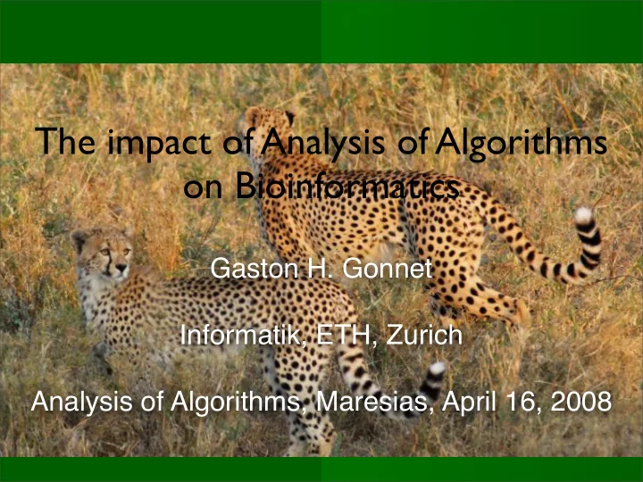
The impact of Analysis of Algorithms on Bioinformatics Gaston H. Gonnet Informatik, ETH, Zurich Analysis of Algorithms, Maresias, April 16, 2008 Abstract In principle, Analysis of Algorithms and Bioinformatics share few tools and methods.
The impact of Analysis of Algorithms on Bioinformatics Gaston H. Gonnet Informatik, ETH, Zurich Analysis of Algorithms, Maresias, April 16, 2008
Abstract In principle, Analysis of Algorithms and Bioinformatics share few tools and methods. This is only true when we look at the surface, deeper inspection shows many points of convergence, in particular in asymptotic analysis and model development. We would also like to stress the importance and usefulness of Maximum Likelihood for modelling in bioinformatics and the relation to problems in Analysis of Algorithms. .
Bertioga to Sao Sebastiao in 1971
Bertioga to Sao Sebastiao in 1971
Central Dogma of Molecular Evolution
Double stranded DNA is reproduced
Modelling Analysis of Algorithms gives us a natural ability to model and analyze processes. What makes a good model? Must capture the essence of the process As simple as possible, but not simpler Realistic in terms of the application Analyzable
Modelling: Closed form vs computational Simple models may allow closed form solutions, more realistic (complicated) models may only allow numerical solutions A closed form solution gives you insight! Numerical computation gives you results which can be used.
Mistakes happen during DNA replication Most mistakes are harmful, give the organism a disadvantage and it does not survive/compete. Some mistakes are irrelevant, i.e. do not cause any difference. Rarely they remain in the population. Some mistakes are helpful they either improve the organism or adapt it better to the environment. These are very likely to survive in the population.
Mistakes modeled as a Markovian process The occurrence and complicated acceptance of DNA mutations is modeled as a Markov process This is known to be flawed, but still is the best model for DNA/protein evolution A C G T A 0.93 0.01 0.07 0.01 C 0.02 0.95 0.02 0.02 M = G 0.03 0.01 0.88 0.01 T 0.02 0.03 0.03 0.96
Mutation matrices Mp 0 = p 1 M defines a unit of mutation Infinite mutation results in the M ∞ p = f natural (default) frequencies f is the eigenvector with Mf = f eigenvalue 1 of M
Mutation matrices (II) Q is the rate (differential M d = e dQ equations of transitions) matrix Eigenvalue/eigenvector Q = U Λ U − 1 decomposition of Q M d = Ue d Λ U − 1 λ 1 = 0 , U 1 = f from Mf=f λ i < 0 , i > 1 reaches steady state
The principle of Molecular evolution Dog DNA Elephant DNA Rabbit DNA aactgagcggtt... aactgacccggtt... aactgaccggtt...
Phylogenetic tree of 17 vertebrates BRARE TETNG FUGRU XENTR CHICK MONDO MOUSE RATNO ECHTE LOXAF DASNO BOVIN 96% CANFA 85% RABIT Amphibia 99.0% MACMU Sauropsida Metatheria PANTR Actinopterygii HUMAN Eutheria BestDimless Tree of 17 Vertebrates, (C) 2006 CBRG, ETH Zurich
Tree of mammals
Probabilities vs likelihoods Some event For particular Over all X, A data, as a and B defines function of d, a probability defines a space likelihood
Maximum likelihood (I) How to estimate parameters by Maximum likelihood? Compute the likelihood, or log of the likelihood, and maximize L ( θ ) = Prob { event depending on θ } i Prob { i th event depending on θ } L ( θ ) = � i ln(Prob { i th event depending on θ } ) ln( L ( θ )) = �
Maximum likelihood (II) max( L ( θ )) = L (ˆ θ ) L ′ (ˆ θ ) θ ) = 0 L (ˆ L ′′ (ˆ θ ) 1 θ ) = − L (ˆ σ 2 (ˆ θ ) Also applicable to vectors with the usual matrix interpretations
Maximum likelihood (III) Completely analogous to the asymptotic estimation of integrals based on the approximation of the maximum by a 0 e − a 1 x 2
Maximum likelihood (IV) The maximum likelihood estimators are: Unbiased Most efficient (of the unbiased estimators, the ones with smallest variance) Normally distributed
Maximum likelihood (V) This is ideal for symbolic/numeric computation Complicated problems/models can be stated in their most natural form The literature usually warns against the difficulty of computing derivatives and solving non-linear equations (maximum) ????
Some people have not discovered symbolic computation yet... There are only two drawbacks to MLE’s, but they are important ones: • With small numbers of failures (less than 5, and sometimes less than 10 is small), MLE’s can be heavily biased and the large sample optimality properties do not apply • Calculating MLE’s often requires specialized software for solving complex non-linear equations. This is less of a problem as time goes by, as more statistical packages are upgrading to contain MLE analysis capability every year.
Inter sequence distance estimation by ML s A A C T T G C G G d t A C C T G G C G C i ( M d ) s i ,t i L ( d ) = � i ln(( M d ) s i ,t i ) ln( L ( d )) = �
Inter sequence distance estimation by ML i ln(( M d ) s i ,t i ) ln( L ( d )) = � This is normally called the score of an alignment and it is used (with some normalization) by the dynamic programming algorithm for sequence alignment
Inter sequence distance estimation by ML 3200 3000 2800 2600 2400 2200 2000 1800 1600 1400 1200 20 40 60 80 100 120 140 160 180 200 220 240 Score (likelihood) vs PAM distance for a particular protein alignment
Estimation of deletion costs by ML The Zipfian model of indels postulates that indels have a probability given by: 1 Pr { indel of length k } = c 0 ( d ) ζ ( θ ) k θ where the first term is the probability of opening an indel and the second gives the distribution of indels according to length
Estimation of deletion costs by ML (II) Empirically: ln( c 0 ( d )) = d 0 + d 1 ln( d ) which means that the score of an indel is modeled by the formula: ln(indel length k ) = d 0 + d 1 ln( d ) − θ ln k a model with 3 unknown parameters
Estimation of deletion costs by ML (III) Collecting information from gaps in real alignments (thousands of them) we can fit these parameters by maximum likelihood
Recommend
More recommend
Explore More Topics
Stay informed with curated content and fresh updates.
