The Geometry of Least Squares Mathematical Basics Inner / dot - PowerPoint PPT Presentation
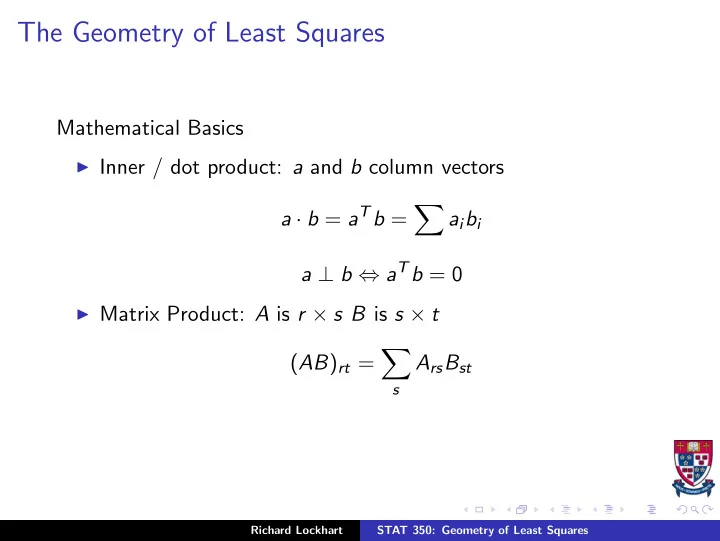
The Geometry of Least Squares Mathematical Basics Inner / dot product: a and b column vectors a b = a T b = a i b i a b a T b = 0 Matrix Product: A is r s B is s t ( AB ) rt = A rs B st s Richard Lockhart STAT
The Geometry of Least Squares Mathematical Basics ◮ Inner / dot product: a and b column vectors � a · b = a T b = a i b i a ⊥ b ⇔ a T b = 0 ◮ Matrix Product: A is r × s B is s × t � ( AB ) rt = A rs B st s Richard Lockhart STAT 350: Geometry of Least Squares
Partitioned Matrices ◮ Partitioned matrices are like ordinary matrices but the entries are matrices themselves. ◮ They add and multiply (if the dimensions match properly) just like regular matrices but(!) you must remember that matrix multiplication is not commutative. ◮ Here is an example � A 11 � A 12 A 13 A = A 21 A 22 A 23 B 11 B 12 B = B 21 B 22 B 31 B 32 Richard Lockhart STAT 350: Geometry of Least Squares
◮ Think of A as a 2 × 3 matrix and B as a 3 × 2 matrix. ◮ multiply them to get C = AB a 2 × 2 matrix as follows: � A 11 B 11 + A 12 B 21 + A 13 B 31 � A 11 B 12 + A 12 B 22 + A 13 B 32 AB = A 21 B 11 + A 22 B 21 + A 23 B 31 A 21 B 12 + A 22 B 22 + A 23 B 32 ◮ BUT: this only works if each of the matrix products in the formulas makes sense. ◮ So, A 11 must have the same number of columns as B 11 has rows and many other similar restrictions apply. Richard Lockhart STAT 350: Geometry of Least Squares
First application: X = [ X 1 | X 2 | · · · | X p ] where each X i is a column of X . Then β 1 . . X β = [ X 1 | X 2 | · · · | X p ] = X 1 β 1 + X 2 β 2 + · · · + X p β p . β p which is a linear combination of the columns of X . Definition : The column space of X , written col ( X ) is the (vector space of) set of all linear combinations of columns of X also called the space “spanned” by the columns of X . SO: ˆ µ = X β is in col ( X ). Richard Lockhart STAT 350: Geometry of Least Squares
Back to normal equations: X T Y = X T X ˆ β or X T � � Y − X ˆ β = 0 or X T 1 � � . Y − X ˆ . β = 0 . X T p or � � Y − X ˆ X T = 0 i = 1 , . . . , p β i or Y − X ˆ β ⊥ every vector in col ( X ) Richard Lockhart STAT 350: Geometry of Least Squares
ǫ = Y − X ˆ Definition : ˆ β is the fitted residual vector. SO: ˆ ǫ ⊥ col ( X ) and ˆ ǫ ⊥ ˆ µ Pythagoras’ Theorem : If a ⊥ b then || a || 2 + || b || 2 = || a + b || 2 Definition : || a || is the “length” or “norm” of a : √ �� a 2 || a || = i = a T a Moreover, if a , b , c , . . . are all perpendicular then || a || 2 + || b || 2 + · · · = || a + b + · · · || 2 Richard Lockhart STAT 350: Geometry of Least Squares
Application Y = Y − X ˆ β + X ˆ β = ˆ ǫ + ˆ µ so || Y || 2 = || ˆ ǫ || 2 + || ˆ µ || 2 or � � � Y 2 ǫ 2 µ 2 i = ˆ i + ˆ i Definitions : � Y 2 i = Total Sum of Squares (unadjusted) � ǫ 2 ˆ i = Error or Residual Sum of Squares � µ 2 ˆ i = Regression Sum of Squares Richard Lockhart STAT 350: Geometry of Least Squares
Alternative formulas for the Regression SS � µ T ˆ µ 2 ˆ i = ˆ µ = ( X ˆ β ) T ( X ˆ β ) β T X T X ˆ = ˆ β Notice the matrix identity which I will use regularly: ( AB ) T = B T A T . Richard Lockhart STAT 350: Geometry of Least Squares
What is least squares? Choose ˆ β to minimize � µ i ) 2 = || Y − ˆ µ || 2 ( Y i − ˆ ǫ || 2 . The resulting ˆ That is, to minimize || ˆ µ is called the Orthogonal Projection of Y onto the column space of X . Extension : � β 1 � X = [ X 1 | X 2 ] β = p = p 1 + p 2 β 2 Imagine we fit 2 models: 1. The FULL model: Y = X β + ǫ (= X 1 β 1 + X 2 β 2 + ǫ ) 2. The REDUCED model: Y = X 1 β 1 + ǫ Richard Lockhart STAT 350: Geometry of Least Squares
If we fit the full model we get ˆ ˆ ˆ ˆ ǫ F ⊥ col ( X ) (1) β F µ F ǫ F If we fit the reduced model we get ˆ ˆ ˆ ˆ µ R ∈ col ( X 1 ) ⊂ col ( X ) (2) β R µ R ǫ R Notice that ˆ ǫ F ⊥ ˆ (3) µ R . (The vector ˆ µ R is in the column space of X 1 so it is in the column space of X and ˆ ǫ F is orthogonal to everything in the column space of X .) So: Y = ˆ ǫ F + ˆ µ F = ˆ ǫ F + ˆ µ R + (ˆ µ F − ˆ µ R ) = ǫ R + ˆ µ R Richard Lockhart STAT 350: Geometry of Least Squares
You know ˆ ǫ F ⊥ ˆ µ R (from (3) above) and ˆ ǫ F ⊥ ˆ µ F (from (1) above). So ǫ F ⊥ ˆ ˆ µ F − ˆ µ R Also µ R ⊥ ˆ ˆ ǫ R = ˆ ǫ F + (ˆ µ F − ˆ µ R ) So µ R ) T ˆ 0 = (ˆ ǫ F + ˆ µ F − ˆ µ R µ R ) T ˆ ǫ T = ˆ F ˆ µ R +(ˆ µ F − ˆ µ R � �� � 0 so µ F − ˆ ˆ µ R ⊥ ˆ µ R Richard Lockhart STAT 350: Geometry of Least Squares
Summary We have Y = ˆ µ R + (ˆ µ F − ˆ µ R ) + ˆ ǫ F All three vectors on the Right Hand Side are perpendicular to each other. This gives: || Y || 2 = || ˆ µ R || 2 + || ˆ µ R || 2 + || ˆ ǫ F || 2 µ F − ˆ which is an Analysis of Variance (ANOVA) table! Richard Lockhart STAT 350: Geometry of Least Squares
Here is the most basic version of the above: X = [ 1 | X 1 ] Y i = β 0 + · · · + ǫ i The notation here is that 1 . . 1 = . 1 is a column vector with all entries equal to 1. The coefficient of this column, β 0 , is called the “intercept” term in the model. Richard Lockhart STAT 350: Geometry of Least Squares
To find ˆ µ R we minimize � ( Y i − ˆ β 0 ) 2 and get simply β 0 = ¯ ˆ Y and ¯ Y . . µ R = ˆ . ¯ Y Our ANOVA identity is now || Y || 2 = || ˆ µ R || 2 + || ˆ µ R || 2 + || ˆ ǫ F || 2 µ F − ˆ Y 2 + || ˆ µ R || 2 + || ˆ = n ¯ ǫ F || 2 µ F − ˆ Richard Lockhart STAT 350: Geometry of Least Squares
This identity is usually rewritten in subtracted form: || Y || 2 − n ¯ Y 2 = || ˆ µ R || 2 + || ˆ ǫ F || 2 µ F − ˆ Y ) 2 = � Y 2 Y 2 we find Remembering the identity � ( Y i − ¯ i − n ¯ � � � Y ) 2 = Y ) 2 + ( Y i − ¯ µ F , i − ¯ ǫ 2 (ˆ ˆ F , i These terms are respectively: ◮ the Adjusted or Corrected Total Sum of Squares, ◮ the Regression or Model Sum of Squares and ◮ the Error Sum of Squares. Richard Lockhart STAT 350: Geometry of Least Squares
Simple Linear Regression ◮ Filled Gas tank 107 times. ◮ Record distance since last fill, gas needed to fill. ◮ Question for discussion: natural model? ◮ Look at JMP analysis. Richard Lockhart STAT 350: Geometry of Least Squares
The sum of squares decomposition in one example ◮ Example discussed in Introduction . ◮ Consider model Y ij = µ + α i + ǫ ij with α 4 = − ( α 1 + α 2 + α 3 ). ◮ Data consist of blood coagulation times for 24 animals fed one of 4 different diets. ◮ Now I write the data in a table and decompose the table into a sum of several tables. ◮ The 4 columns of the table correspond to Diets A, B, C and D. ◮ You should think of the entries in each table as being stacked up into a column vector, but the tables save space. Richard Lockhart STAT 350: Geometry of Least Squares
◮ The design matrix can be partitioned into a column of 1s and 3 other columns. ◮ You should compute the product X T X and get 24 − 4 − 2 − 2 − 4 12 8 8 − 2 8 14 8 − 2 8 8 14 ◮ The matrix X T Y is just � � � � � � � Y ij , Y 1 j − Y 4 j , Y 2 j − Y 4 j , Y 3 j − Y 4 j ij j j j j j j Richard Lockhart STAT 350: Geometry of Least Squares
◮ The matrix X T X can be inverted using a program like Maple. ◮ I found that 17 7 − 1 − 1 7 65 − 23 − 23 384( X T X ) − 1 = − 1 − 23 49 − 15 − 1 − 23 − 15 49 ◮ It now takes quite a bit of algebra to verify that the vector of fitted values can be computed by simply averaging the data in each column. Richard Lockhart STAT 350: Geometry of Least Squares
That is, the fitted value, ˆ µ is the table 61 66 68 61 61 66 68 61 61 66 68 61 61 66 68 61 66 68 61 66 68 61 61 61 Richard Lockhart STAT 350: Geometry of Least Squares
On the other hand fitting the model with a design matrix consisting only of a column of 1s just leads to ˆ µ R (notation from the lecture) given by 64 64 64 64 64 64 64 64 64 64 64 64 64 64 64 64 64 64 64 64 64 64 64 64 Richard Lockhart STAT 350: Geometry of Least Squares
Earlier I gave identity: Y = ˆ µ R + (ˆ µ F − ˆ µ R ) + ˆ ǫ F which corresponds to the following identity: 2 62 63 68 56 3 2 64 64 64 64 3 2 − 3 2 4 − 3 3 2 1 − 3 0 − 5 3 60 67 66 62 64 64 64 64 − 3 2 4 − 3 − 1 1 − 2 1 6 7 6 7 6 7 6 7 6 63 71 71 60 7 6 64 64 64 64 7 6 − 3 2 4 − 3 7 6 2 5 3 − 1 7 6 7 6 7 6 7 6 7 59 64 67 61 64 64 64 64 − 3 2 4 − 3 − 2 − 2 − 1 0 6 7 6 7 6 7 6 7 6 7 = 6 7 + 6 7 + 6 7 65 68 63 64 64 64 2 4 − 3 − 1 0 2 6 7 6 7 6 7 6 7 6 7 6 7 6 7 6 7 66 68 64 64 64 64 2 4 − 3 0 0 3 6 7 6 7 6 7 6 7 6 7 6 7 6 7 6 7 63 64 − 3 2 4 5 4 5 4 5 4 5 59 64 − 3 − 2 Richard Lockhart STAT 350: Geometry of Least Squares
Recommend
More recommend
Explore More Topics
Stay informed with curated content and fresh updates.
