The following chart summarizes which model assumptions are necessary - PowerPoint PPT Presentation
41 42 The following chart summarizes which model assumptions are necessary to prove which part of the theorem: Conclusions about Sampling Distribution out (Distribution of ) 1: Normal 2: Mean 3: Standard rd d d deviation Assumption 1
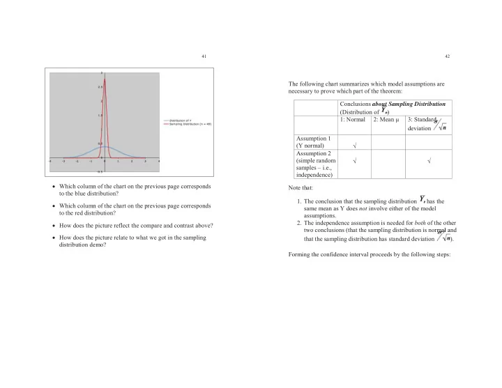
41 42 The following chart summarizes which model assumptions are necessary to prove which part of the theorem: Conclusions about Sampling Distribution out (Distribution of ) 1: Normal 2: Mean μ 3: Standard rd d d deviation Assumption 1 (Y normal) � Assumption 2 (simple random � � samples – i.e., independence) � Which column of the chart on the previous page corresponds Note that: to the blue distribution? 1. The conclusion that the sampling distribution has the � Which column of the chart on the previous page corresponds same mean as Y does not involve either of the model to the red distribution? assumptions. 2. The independence assumption is needed for both of the other � How does the picture reflect the compare and contrast above? two conclusions (that the sampling distribution is normal and rma ma ma m l a a � How does the picture relate to what we got in the sampling that the sampling distribution has standard deviation ). distribution demo? Forming the confidence interval proceeds by the following steps:
43 44 1. First, we specify some high degree of probability; this called the Robustness again: confidence level. ( We’ll use 0.95 to illustrate; so we’ll say “95% confidence level.”) In practice we can’t find a exactly for this procedure, since we 2. The first two conclusions of the theorem (that the sampling onc don’t know � . distribution of is normal with mean μ ) imply that there is � But using the sample standard deviation s to approximate number a so that � will give a good approximation. (*) The probability that lies between μ - a and μ + a is � And, once we actually have a sample, we will know the 0.95: value of n, so we can use a t-distribution to find a more < μ + a) �� 0.95 P( μ - a < precise value for a for that sample size. [Draw a picture of the sampling distribution to help see why!] � Many procedures are “exact” (that is, don’t require an approximation), but the additional complications they involve make this procedure better for explaining the basic idea. Caution : It’s important to keep in mind what is a random variable and what is a constant: � Is μ a constant or a random variable? _______________ � Is a a constant or a random variable? ________________ a a � Is a constant or a random variable? ________________ Here, the random variable is in the middle of the interval, which is what makes the most sense in a probability statement. All is good!
45 46 3. A little algebraic manipulation (which can be stated in words as, “If the estimate is within a units of the mean μ , then μ is within a units of the estimate”) allows us to restate (*) as (**) The probability that μ lies between - a and + a is approximately 0.95: app p y 0 + a) is approximately � 0.95 P( - a < μ < This is looking a strange. Our ONE random variable now appears TWICE in the statement. This is strange for a probability statement, but is still a valid probability statement, because it is exactly the same relationship t, b between , a, and μ as before. http://visualize.tlok.org/elem-stat/mean_confidence_intervals.php On the following page is a picture of the result of taking 100 different simple random samples from a population and using each to form a confidence interval for the mean. (**) The probability that μ lies between - a and + a To create this, we had to know entire population (so that is approximately 0.95: app p y 0 we could repeatedly sample from it, so we knew the mean + a) is approximately � 0.95 P( - a < μ < μ . Notice that the endpoints of the intervals differ, just as the notation says they will. Reinforcement : It’s again important to be clear about what is variable here. That hasn't changed: it’s still the sample that is ple Also notice that not all 100 of them include the actual varying, not μ or a. So the probability still refers to , not to μ . population mean. That is what we expect – we asked for the probability to be 0.95 that an individual confidence Thinking that the probability in (**) refers to μ is a common interval would include the mean. mistake in interpreting confidence intervals. While (**) is a correct statement, as soon as you do the do t obvious next step of putting a sample mean in for so you have numbers at the end of your confidence interval, this is not a probability statement any longer!!!
47 48 We’re now faced with two possibilities (assuming the model Since this is the best we can do, we calculate the values of ce t - a � � assumptions are indeed all true): and + a for the sample we have , and call the resulting interval a 95% confidence interval for μ . 1) The sample we have taken is one of the approximately one e a 95% for which the interval from - a to + a does o We do not say that there is 95% probability that μ is contain μ . � between 48 and 51.5 o We can say that we have obtained the confidence interval 2) Our sample is one of the approximately 5% for which the e is f th by using a procedure that, for approximately 95% of all interval from - a to + a does not contain μ . � simple random samples from Y, of the given size n, produces an interval containing the parameter μ that we Unfortunately, we can't know which of these two possibilities � are estimating. is true for the sample we have. � o Unfortunately, we can't know whether or not the sample So we are left with some (more) uncertainty. � we’ve used is one of the approximately 95% of "nice" samples that yield a confidence interval containing the true mean μ , or whether the sample we have is one of the approximately 5% of "bad" samples that yield a confidence interval that does not contain the true mean μ . o We can just say that we have used a procedure that "works" about 95% of the time. o In other words, “confidence” is in the degree of reliability of the method* , not of the result. *“The method” here refers to the entire process: Choose sample � Record values of Y for sample � Calculate confidence interval.
49 50 Variations and trade-offs: I hope this convinces you that: We can decide on the "level of confidence" we want; � � A result based on a single sample could be wrong, even if the analysis is carefully carried out! o E.g., we can choose 90%, 99%, etc. rather than 95%. � Consistent results from careful analyses of several o Just which level of confidence is appropriate depends on independently collected samples would be more convincing. the circumstances. (More later) � I.e., replication of studies, using independent samples, is important! ( More on this later.) The confidence level is the proportion (expressed as a � percentage) of samples for which the procedure results in an In general: We can follow a similar procedure for many other interval containing the true parameter. (Or approximate situations to obtain confidence intervals for parameters. proportion, if the procedure is not exact.) Each type of confidence interval procedure has its own model However, a higher level of confidence will produce a wider � � assumptions. confidence interval . o If the model assumptions are not true, we can’t be sure o i.e., less certainty in our estimate. that the procedure does what is claimed . o So there is a trade-off between level of confidence and o However, some procedures are robust to some degree to degree of certainty . (No free lunch!) some departures from models assumptions -- i.e., the Sometimes the best we can do is a procedure that only gives � procedure works pretty closely to what is intended if the approximate confidence intervals. model assumption is not too far from true. o i.e., the sampling distribution can be described only o As with hypothesis tests, robustness depends on the approximately. particular procedure; there are no "one size fits all" rules. o i.e., there is one more source of uncertainty. No matter what the procedure is, replication is still � important! o This is the case for the large-sample z-procedure. Note : If the sampling distribution is not symmetric, we can't � expect the confidence interval to be symmetric around the estimate.
Recommend
More recommend
Explore More Topics
Stay informed with curated content and fresh updates.


