The exchange value embedded in a transport system Qinglan Xia - PowerPoint PPT Presentation
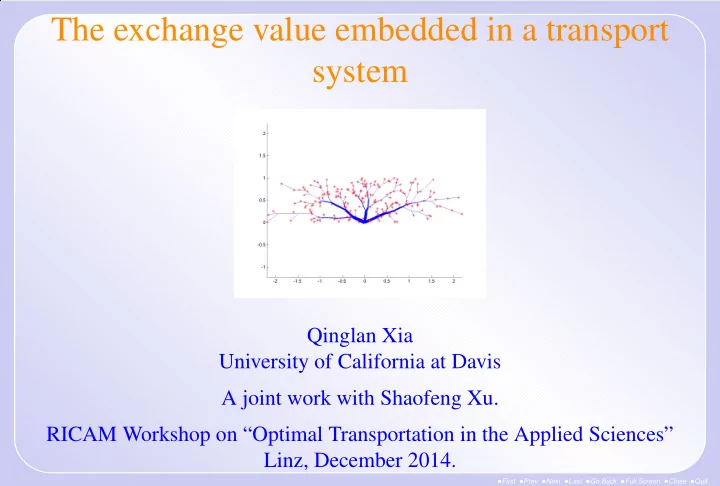
The exchange value embedded in a transport system Qinglan Xia University of California at Davis A joint work with Shaofeng Xu. RICAM Workshop on Optimal Transportation in the Applied Sciences Linz, December 2014. First Prev
The exchange value embedded in a transport system Qinglan Xia University of California at Davis A joint work with Shaofeng Xu. RICAM Workshop on “Optimal Transportation in the Applied Sciences” Linz, December 2014. • First • Prev • Next • Last • Go Back • Full Screen • Close • Quit
Ramified optimal transportation Ramified optimal transportation is a closely related (but different) type of transportation to the Monge-Kantorovich problem. It aims at modeling a tree-shaped branching transport system via an optimal transport path between two probability measures. Ramified optimal transportation problem: minimize � θ ( x ) α d H 1 ( x ) M α ( T ) := spt ( T ) among all transport path T ∈ Path ( µ + , µ − ) , which is a rectifiable 1-current with ∂T = µ − − µ + . • First • Prev • Next • Last • Go Back • Full Screen • Close • Quit
Example: transport between atomic measures Consider two atomic measures k ℓ � � a = m i δ x i and b = n j δ y j i =1 j =1 with k ℓ � � m i = n j = 1 . i =1 j =1 a A transport path from a to b is a polyhe- dral chain G with boundary ∂G = b − a . V b • First • Prev • Next • Last • Go Back • Full Screen • Close • Quit
Cost Functionals For each G = { V ( G ) , E ( G ) , w : E ( G ) → (0 , + ∞ ) } , define the M α mass of G by w ( e ) α length ( e ) � M α ( G ) := e ∈ E ( G ) for some α ∈ [0 , 1) . Here, the length of any edge e is the Euclidean distance between its end- points. • First • Prev • Next • Last • Go Back • Full Screen • Close • Quit
• First • Prev • Next • Last • Go Back • Full Screen • Close • Quit
• First • Prev • Next • Last • Go Back • Full Screen • Close • Quit
• First • Prev • Next • Last • Go Back • Full Screen • Close • Quit
• First • Prev • Next • Last • Go Back • Full Screen • Close • Quit
• First • Prev • Next • Last • Go Back • Full Screen • Close • Quit
• First • Prev • Next • Last • Go Back • Full Screen • Close • Quit
• First • Prev • Next • Last • Go Back • Full Screen • Close • Quit
• First • Prev • Next • Last • Go Back • Full Screen • Close • Quit
• First • Prev • Next • Last • Go Back • Full Screen • Close • Quit
• First • Prev • Next • Last • Go Back • Full Screen • Close • Quit
• First • Prev • Next • Last • Go Back • Full Screen • Close • Quit
• First • Prev • Next • Last • Go Back • Full Screen • Close • Quit
• First • Prev • Next • Last • Go Back • Full Screen • Close • Quit
• First • Prev • Next • Last • Go Back • Full Screen • Close • Quit
• First • Prev • Next • Last • Go Back • Full Screen • Close • Quit
• First • Prev • Next • Last • Go Back • Full Screen • Close • Quit
• First • Prev • Next • Last • Go Back • Full Screen • Close • Quit
• First • Prev • Next • Last • Go Back • Full Screen • Close • Quit
Transport plan Recall that a transport plan from a to b is an atomic probability measure k ℓ � � q = q ij δ ( x i ,y j ) (1) i =1 j =1 on the product space X × X such that for each i and j , q ij ≥ 0 , k ℓ � � q ij = n j and q ij = m i . (2) i =1 j =1 Denote Plan ( a , b ) as the space of all transport plans from a to b . In a transport plan q , the number q ij denotes the amount of commodity re- ceived by household j from factory i . • First • Prev • Next • Last • Go Back • Full Screen • Close • Quit
A matrix associated with a transport path Let G be a transport path in Path ( a , b ) . We assume that for each x i and y j , there exists at most one directed polyhedral curve g ij from x i to y j . In other words, there exists a list of distinct vertices � � � � v i 1 , v i 2 , · · · , v i h V g ij := (3) � � in V ( G ) with x i = v i 1 , y j = v i h , and each v i t , v i t +1 is a directed edge in E ( G ) for each t = 1 , 2 , · · · , h − 1 . This assumption clearly holds when G contains no cycles. For some pairs of ( i, j ) , such a curve g ij from x i to y j may fail to exist, due to reasons like geographical barriers, law restrictions, etc. If such curve does not exist, we set g ij = 0 to denote the empty directed polyhedral curve. By doing so, we construct a matrix � � g = g ij (4) k × ℓ with each element of g being a polyhedral curve. • First • Prev • Next • Last • Go Back • Full Screen • Close • Quit
A simple example A transport path from 4 δ x 1 + 3 δ x 2 + 4 δ x 3 to 3 δ y 1 + 5 δ y 2 + 3 δ y 3 with g 13 = 0 , g 31 = 0 . � � For any transport path G ∈ Path ( a , b ) , such a matrix g = g ij is uniquely determined. • First • Prev • Next • Last • Go Back • Full Screen • Close • Quit
Compatibility between plan and path Let G ∈ Path ( a , b ) be a transport path and q ∈ Plan ( a , b ) be a transport plan. The pair ( G, q ) is compatible if q ij = 0 whenever g ij = 0 and G = q · g. (5) Here, equation (5) means that as polyhedral chains, k ℓ � � q ij · g ij , G = i =1 j =1 where the product q ij · g ij denotes that an amount q ij of commodity is moved along the polyhedral curve g ij from factory i to household j . In terms of edges, it says that for each edge e ∈ E ( G ) , we have � q ij = w ( e ) . e ⊆ g ij • First • Prev • Next • Last • Go Back • Full Screen • Close • Quit
Compatible pair of transport path and plan For instance, the transport path in previous example can be expressed as G = 2 g 11 + 2 g 12 + g 21 + g 22 + g 23 + 2 g 32 + 2 g 33 , (6) which means that the transport plan q = 2 δ (1 , 1) + 2 δ (1 , 2) + δ (2 , 1) + δ (2 , 2) + δ (2 , 3) + 2 δ (3 , 2) + 2 δ (3 , 3) is compatible with G in (6). • First • Prev • Next • Last • Go Back • Full Screen • Close • Quit
Example Roughly speaking, the compatibility conditions check whether a transport plan is realizable by a transport path. a =1 4 δ x 1 + 3 4 δ x 2 and b =5 8 δ y 1 + 3 8 δ y 2 , and consider a transport plan q = 1 8 δ ( x 1 ,y 1 ) + 1 8 δ ( x 1 ,y 2 ) + 1 2 δ ( x 2 ,y 1 ) + 1 4 δ ( x 2 ,y 2 ) ∈ Plan ( a , b ) . (7) It is straight forward to see that q is compatible with G 1 but not G 2 . This is because there is no directed curve g 12 from factory 1 to household 2 in G 2 . • First • Prev • Next • Last • Go Back • Full Screen • Close • Quit
A transport path ¯ G compatible with all plans Example. Let x ∗ ∈ X \ { x 1 , · · · , x k , y 1 , · · · , y ℓ } . We may construct a path ¯ G ∈ Path ( a , b ) as follows. Let � ¯ = { x 1 , · · · , x k } ∪ { y 1 , · · · , y ℓ } ∪ { x ∗ } , � V G � ¯ = { [ x i , x ∗ ] : i = 1 , · · · , k } ∪ x ∗ , y j � �� � � E G : j = 1 , · · · , ℓ , and w ([ x i , x ∗ ]) = m i , w x ∗ , y j �� �� = n j for each i and j . In this case, each g ij is the union of two edges [ x i , x ∗ ] ∪ x ∗ , y j . Then, each transport plan q ∈ Plan ( a , b ) is compatible with ¯ � � G . • First • Prev • Next • Last • Go Back • Full Screen • Close • Quit
Motivations As an illustration, we consider a spacial economy with two goods located at two distinct points { x 1 , x 2 } and two consumers living at two different locations { y 1 , y 2 } . • Consumer 1 favors good 2 more than good 1. However, good 2 may be more expensive than good 1 for some reason such as a higher transporta- tion fee. • As a result, she buys good 1 despite the fact that it is not her favorite. • On the contrary, consumer 2 favors good 1 but ends up buying good 2, as good 1 is more expensive than good 2 for him. • First • Prev • Next • Last • Go Back • Full Screen • Close • Quit
Motivations Given this purchase plan, a traditional trans- porter will ship the ordered items in a trans- port system like G 1 . However, in ramified (i.e. branching) optimal transportation, a transport system like G 2 with some branching structure might be more cost efficient than G 1 . One may save some trans- portation cost by using a transport system like G 2 instead of G 1 . Advantage of G 2 over G 1 : • G 2 might be more cost efficient than G 1 : one may save some transportation cost by using a transport system like G 2 instead of G 1 . • Now, we observe another very interesting advantage about G 2 . • First • Prev • Next • Last • Go Back • Full Screen • Close • Quit
Exchange: a happier life for free! Unlike a traditional transport system G 1 , a ramified transport system G 2 pro- vides an exchange value: one can simply switch the items which leads to consumer 1 getting good 2 and consumer 2 receiving good 1. • This exchange of items makes both consumers better off since they both get what they prefer. • More importantly, no extra transportation cost is incurred during this ex- change process. In other words, a ramified transport system like G 2 may possess an exchange value, which cannot be found in a traditional transport system G 1 . How shall we quantify the exchange value for a ramified transport system? • First • Prev • Next • Last • Go Back • Full Screen • Close • Quit
Recommend
More recommend
Explore More Topics
Stay informed with curated content and fresh updates.


