The dynamics of infectious disease outbreaks Jonathan Dushoff - PowerPoint PPT Presentation
The dynamics of infectious disease outbreaks Jonathan Dushoff McMaster University Department of Biology Seminar Series Feb 2020 Novel Coronavirus: What do we need to know? How deadly is the disease? Can spread be stopped? What
Example: Post-death transmission and safe burial ◮ How much Ebola spread occurs before vs. after death ◮ Highly context dependent ◮ Funeral practices, disease knowledge ◮ Weitz and Dushoff Scientific Reports 5:8751.
Conditional effect of generation time ◮ Given the reproductive number R ◮ faster generation time G means higher r ◮ More danger ◮ Given r ◮ faster generation time G means smaller R ◮ Less danger
Linking framework ◮ Epidemic speed r is a product : ◮ (something to do with) generation speed ◮ × (something to do with) epidemic strength ◮ Epidemic strength R is therefore (approximately) a quotient ◮ Epidemic speed ◮ ÷ (something to do with) generation speed
Effect of variation in generation time ◮ For a given value of mean generation time, what happens if we have more variation in generation time? ◮ Events that happen earlier than expected compound through time ◮ If R is fixed then r will be higher = ⇒ ◮ If r is fixed then R will be lower
Approximations Approximate generation intervals Effective reproductive number R 5 0.04 4 Density (1/day) 3 0.02 2 0.00 1 0 10 20 30 40 50 0.5 1.0 1.5 2.0 Generation interval (days) Exponential growth rate (per generation)
Moment approximation Approximate generation intervals Effective reproductive number R 0.06 5 4 Density (1/day) 0.04 3 0.02 2 0.00 1 0 10 20 30 40 50 0.5 1.0 1.5 2.0 Generation interval (days) Exponential growth rate (per generation)
Moment approximation Approximate generation intervals 0.08 Effective reproductive number R 5 0.06 4 Density (1/day) 0.04 3 0.02 2 0.00 1 0 10 20 30 40 50 0.5 1.0 1.5 2.0 Generation interval (days) Exponential growth rate (per generation)
Moment approximation Approximate generation intervals Effective reproductive number R 5 0.08 4 Density (1/day) 3 0.04 2 0.00 1 0 10 20 30 40 50 0.5 1.0 1.5 2.0 Generation interval (days) Exponential growth rate (per generation)
Approximation framework ◮ R ≈ X ( r ¯ G ; 1 /κ ) ◮ κ is the dispersion parameter of the generation-interval distribution (measures the effective amount of variation ◮ X is the compound-interest function ◮ R ≈ 1 + r ¯ G when variation is large ◮ R ≈ exp( r ¯ G ) when variation is small ◮ Key quantity is r ¯ G : the relative length of the generation interval compared to the characteristic time scale of spread
Intuition ◮ Longer generation times mean less speed = ⇒ more strength, when speed is fixed ◮ ◮ What about more variation in generation times? ◮ More action (both before and after the mean time) ◮ But what happens early is more important in a growing system ◮ More variation means more speed ◮ = ⇒ less strength, when speed is fixed
Test the approximations ◮ Simulate realistic generation intervals for various diseases ◮ Compare approximate r R relationship with known exact relationship ◮ Known because we are testing ourselves with simulated data
Ebola distribution Lognormal SEIR Single−gamma approximation 0.06 0.06 0.04 0.04 Density Density 0.02 0.02 0.00 0.00 0 20 40 60 80 0 20 40 60 80 Generation interval (days) Generation interval (days)
Ebola curve 5 Effective reproductive number R 4 3 2 ● ● ● 1 0.5 1.0 1.5 2.0 Exponential growth rate (per generation)
Measles curve empirical approximation theory (moment) Reproduction number 20 ● Biologically realistic range (12.5 − 18) ● 10 0 0 1 2 3 Relative length of generation interval ( ρ )
Rabies curve empirical approximation theory (moment) approximation theory (MLE) 2.5 Reproduction number 2.0 1.5 Serengeti Ngorongoro ● ● 1.0 0.00 0.25 0.50 0.75 1.00 0 100 200 Relative length of generation interval ( ρ ) Generation interval (days)
Outline How deadly? Dynamical modeling Speed and strength Epidemic Epidemic strength Linking Propagating error in novel coronavirus A false dichotomy Measuring generation intervals
Assumptions
Assumptions
Assumptions
Propagating error A. Baseline 4.5 4.0 Basic reproductive number 3.5 3.0 ● ● ● ● ● 2.5 2.0 base growth rate GI mean growth rate all + GI mean Uncertainty type
Propagating error B. Reduced uncertainty in the growth rate 3.4 Basic reproductive number 3.0 ● ● ● ● ● 2.6 base growth rate GI mean growth rate all + GI mean Uncertainty type
Outline How deadly? Dynamical modeling Speed and strength Epidemic Epidemic strength Linking Propagating error in novel coronavirus A false dichotomy Measuring generation intervals
A false dichotomy ◮ Why are people scrambling to estimate R and mostly ignoring r ? ◮ History ◮ Modelers gotta model
The strength paradigm ◮ R > 1 is a threshold ◮ If we can reduce transmission by a constant factor of θ > R , disease can be controlled ◮ In general, we can define θ as a (harmonic) mean of the reduction factor over the course of an infection ◮ weighted by the intrinsic generation interval ◮ Epidemic is controlled if θ > R ◮ More useful in long term (tells us about final size, equilibrium)
The speed paradigm ◮ r > 0 is a threshold ◮ If we can reduce transmission at a constant hazard rate of φ > r , disease can be controlled ◮ In general, we can define φ as a (very weird) mean of the reduction factor over the course of an infection ◮ weighted by the backward generation interval ◮ Epidemic is controlled if φ > r ◮ More useful in short term (tells us about, um, speed)
Epidemic strength (present) Ebola 0.12 0.10 0.08 Density (1/days) ◮ R , the epidemic 0.06 strength, is the area under the curve. 0.04 0.02 0.00 0 10 20 30 40 time (days)
Strength of intervention Ebola 0.12 0.10 0.08 ◮ . . . by what factor do I Density (1/days) need to reduce this 0.06 curve to eliminate the 0.04 epidemic? 0.02 0.00 0 10 20 30 40 time (days)
Different interventions (present) Ebola 0.12 0.10 0.08 ◮ idealized vaccination Density (1/days) 0.06 ◮ removes a fixed 0.04 proportion of people 0.02 0.00 0 10 20 30 40 time (days)
Different interventions (present) Ebola 0.12 0.10 0.08 ◮ idealized quarantine Density (1/days) 0.06 ◮ removes people at a 0.04 fixed rate 0.02 0.00 0 10 20 30 40 time (days)
Epidemic speed Ebola 0.12 0.10 0.08 ◮ r , the epidemic speed, Density (1/days) is the “discount” rate 0.06 required to balance the 0.04 tendency to grow 0.02 0.00 0 10 20 30 40 time (days)
Epidemic speed Ebola 0.12 0.10 0.08 ◮ k ( τ ) = exp( r τ ) b ( τ ), Density (1/days) where b ( τ ) is the initial 0.06 backward generation 0.04 interval 0.02 0.00 0 10 20 30 40 time (days)
Speed of intervention Ebola 0.12 0.10 0.08 ◮ . . . how quickly do I Density (1/days) need to reduce this 0.06 curve to eliminate the 0.04 epidemic? 0.02 0.00 0 10 20 30 40 time (days)
Different interventions (present) Ebola 0.12 0.10 0.08 Density (1/days) ◮ Sometimes it’s easier to 0.06 estimate strength, sometimes speed 0.04 0.02 0.00 0 10 20 30 40 time (days)
Measuring the intervention
HIV ◮ The importance of transmission speed to HIV control is easier to understand using the speed paradigm ◮ We know the speed of invasion ◮ ≈ 0 . 7 / yr ◮ Characteristic scale ≈ 1 . 4 yr ◮ And can hypothesize the speed of intervention ◮ Or aim to go fast enough
HIV test and treat epidemic 8 intervention 6 Strength 4 2 0 0.10 0.20 0.30 0.40 Early Proportion
HIV test and treat 0.08 0.06 Speed 0.04 0.02 epidemic intervention 0.00 0.10 0.20 0.30 0.40 Early Proportion
Paradigms are complementary ◮ HIV ◮ Information and current intervention are both “speed-like” ◮ Measles ◮ Information (long-term) is strength-like ◮ Intervention (vaccine) also strength-like ◮ Ebola outbreak ◮ Information is speed-like ◮ Pre-emptive vaccination is strength-like ◮ Quarantine or reactive vaccination may be more speed-like
Outline How deadly? Dynamical modeling Speed and strength Epidemic Epidemic strength Linking Propagating error in novel coronavirus A false dichotomy Measuring generation intervals
Measuring generation intervals ◮ Ad hoc methods ◮ Error often not propagated ◮ Importance of heterogeneity
Generations through time ◮ Generation intervals can be estimated by: ◮ Observing patients: ◮ How long does it take to become infectious? ◮ How long does it take to recover? ◮ What is the time profile of infectiousness/activity? ◮ Contact tracing ◮ Who (probably) infected whom? ◮ When did each become infected? ◮ — or ill (serial interval)?
Which is the real interval? ◮ Contact-tracing intervals look systematically different, depending on when you observe them. ◮ Observed in: ◮ Real data, detailed simulations, simple model ◮ Also differ from intrinsic (infector centered) estimates
Types of interval ◮ Define: ◮ Intrinsic interval : How infectious is a patient at time τ after infection? ◮ Forward interval : When will the people infected today infect others? ◮ Backward interval : When did the people who infected people today themselves become infected? ◮ Censored interval : What do all the intervals observed up until a particular time look like? ◮ Like backward intervals, if it’s early in the epidemic
Growing epidemics Liberia ● ● ● ● ● ● ● ● ● ● ● 100 ● ● ● ● ● ● ● ● ● cases ● ● ● ● ● ◮ Generation intervals look shorter 10 at the beginning of an epidemic ● ● ● ◮ A disproportionate number 1 ● ● ● ● of people are infectious right ● ● ● ● ● 2014−01 2014−07 2015−01 now ◮ They haven’t finished all of 0.3 ● ● ● ● ● ● ● ● their transmitting HIV prevalence ● ● ● ● ● ● ◮ We are biased towards 0.2 ● observing faster events ● 0.1 ● ● ● ● ● ● 0.0 1990 2000 2010 Year
Backward intervals Champredon and Dushoff, 2015. DOI:10.1098/rspb.2015.2026
Generations in space ◮ How do local interactions affect realized generation intervals?
Surprising results ◮ We tend to think that heterogeneity leads to underestimates of R , whican can be dangerous. ◮ R on networks generally smaller than values estimated using r . ◮ Trapman et al., 2016. JRS Interface DOI:10.1098/rsif.2016.0288
Generation-interval perspective ◮ Modelers don’t usually question the intrinsic generation interval ◮ But spatial network structure does change generation intervals: ◮ Local interactions = ⇒ wasted contacts ◮ ◮ = ⇒ shorter generation intervals = ⇒ smaller estimates of R . ◮
Observed and estimated intervals homogeneous Intrinsic GI Observed GI in early epidemic assumption • patient-based • contact-tracing based temporal • infectiousness profile of an • censored at observation time infected individual correction local (discount by survival Temporal correction (weight observed periods by exp( rτ )) spatial probability) correction Locally corrected GI Effective GI • based on degree distribution • reflects network structure, but network structure and contact rate [3] corrects for time censoring • depends on between-individual • gives the correct link between r variation and R
Outbreak estimation tracing based empirical individual based Reproductive number 8 4 2 contact population individual empirical egocentric intrinsic tracing correction correction
Serial intervals
Serial intervals ◮ Do serial intervals and generation intervals have the same distribution? ◮ It seems that they should: they describe generations of the same process ◮ But serial intervals can even be very different ◮ Even negative! You might report to the clinic with flu before me, even though I infected you ◮ For rabies, we thought that serial intervals and generation intervals should be the same ◮ Symptoms are closely correlated with infectiousness
Recommend
More recommend
Explore More Topics
Stay informed with curated content and fresh updates.
