The DWR method for numerical simulations related to nuclear waste - PowerPoint PPT Presentation

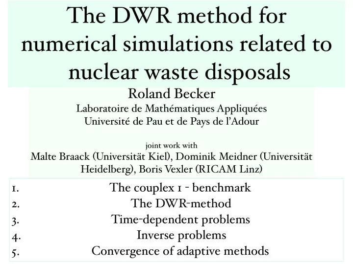
The DWR method for numerical simulations related to nuclear waste disposals Roland Becker Laboratoire de Math é matiques Appliqu é es Universit é de Pau et de Pays de l ’ Adour joint work with Malte Braack ( Universit ä t Kiel ) , Dominik Meidner ( Universit ä t Heidelberg ) , Boris V exler ( RICAM Linz ) The couplex 1 - benchmark 1. The DWR - method 2. Time - dependent problems 3. Inverse problems 4. Convergence of adaptive methods 5.

1. The couplex 1 - benchmark ✤ benchmark de fi nition ✤ our tool: Gascoigne ✤ some thoughts about adaptivity

benchmark de fi nition: couplex 1 ( il manque encore un facteur 3 ) R i ω ( ∂ C i ∂ t + λ i C i ) − ∇ · ( D i ∇ C i ) + u · ∇ C i = f i u = − K ∇ H ∇ · ( K ∇ H ) = 0 + boundary conditions... - linear problem - tremenduous scales - long - time integration - rection - di ff usion - advection with changing regimes

weak formulation Find ( C , H ) in ( C 0 , H 0 )+ V × W such that: a ( C , φ )+ b ( C , H , φ )= l ( φ ) ∀ φ ∈ V d ( H , ψ )= 0 ∀ ψ ∈ W a ( C , φ ) : = � ( C t + λ C ) , φ � + � K ∇ C , ∇φ � b ( C , H , φ ) : = −� K ∇ H · ∇ C , ∇φ � d ( H , ψ ) : = � K ∇ H , ∇ψ � u = ( C , H ) , v = ( φ , ψ ) , X = V × W u ∈ u 0 + X 0 : A ( u , v ) = F ( v ) ∀ v ∈ X

http://www.numerik.uni-kiel.de/~mabr/gascoigne/index.html ✤ adaptive mesh re fi nement ✤ quad ( hex ) - meshes with hanging nodes ✤ Newton, multigrid ✤ fl exibility / modelling ✤ discretization: Q1, Q2 with stabilization

✤ local re fi nement with hanging nodes ✤ multigrid ✤ LPS - local projection stabilization ✦ similar to the schemes of Guermond, Codina, Burman,... [1] R. Becker and M. Braack. A finite element pressure gradient stabilization for the Stokes equations based on local pro jections. Calcolo, 38(4):173–199, 2001.

starting mesh which one to chose ? hydrodynamic load H

adaptive strategy I What quantity ( ies ) to compute ? 1.6 Output requirements The following output quantities are expected from the simulations(both tables and graphical representations): • Contour levels of C i at times 200, 10110, 50110, 10 6 , 10 7 years (the following level values should be used: 10 − 12 , 10 − 10 , 10 − 8 , 10 − 6 , 10 − 4 ); • Pressure field (10 values uniformly distributed between 180 and 340 ; • Darcy velocity field, along the 3 vertical lines given by x = 50 , x = 12500 , x = 20000 , using 100 points along each line; • Places where the Darcy velocity is zero; • Cumulative total flux through the top and the bottom clay layer boundaries, as a function of time; • Cumulative total fluxes through the left boundaries of the dogger and limestone layers; • The discretization grid of the domains and the time stepping used in the simulations should also be given. J ( t )

Γ K ∂ C ( t ) Z J ( t )= ∂ n ds ∂Ω zK ∂ C ( t ) Z = ( z | ∂Ω \ Γ = 0 ) ∂ n ds Z = Ω K ∇ C · ∇ zdx . relates the functional to the operator ! ...

stationary problem ✤ suppose we are interested in mean total fl ux ✤ equations are linear, stationary coe ffi cients ‣ time - derivative drop out Z T J : = 1 0 J ( t ) dt = J ( C ) T Z T C : = 1 0 C ( t ) dt T Find ( C , H ) in ( C 0 , H 0 )+ V × W such that: a ( C , φ )+ b ( C , H , φ )= l ( φ ) ∀ φ ∈ V d ( H , ψ )= 0 ∀ ψ ∈ W

stationary problem ✤ simplify notation: drop overline J ( u ) = A ′ ( u )( u , z ) ≈ F ( z ) − A ( u )( z ) z = ( D , G ) z ∈ z 0 + X a ( φ , D )+ b C ( φ , H , D ) = 0 , A ′ ( u )( v , z ) = 0 ∀ v ∈ X . b H ( C , ψ , D )+ d ( ψ , G ) = 0 . influence sur G

time-averaged solution dual concentration dual pressure

sequence of meshes time - averaged pb

back to the full problem ✤ static adapted meshes ✤ compute dynamic problem on the meshes as above... ✤ what can be said ? how to improve ? ✤ dynamic meshes ✤ needs space - time (fi nite element ) discretization ✤ H needs to be recomputed ✤ adjoint problem is backward in time !!

2. The DWR - method ✤ Task: estimate the ( discretization ) error with respect to a given quantity ✤ Task: automatically construct e ffi cient meshes to compute this quantity idea (1): the quantity is a functional on the solution space

u ∈ V : u h ∈ V h : A ( u , v ) = F ( v ) A ( u h , v ) = F ( v ) ∀ v ∈ V ∀ v ∈ V h suppose linear... ( G ∈ V ∗ ) G ( u ) − G ( u h ) estimate idea ( 2 ) : represent the functional by duality ( c.f. Aubin - Nitsche, Lagrange,... ) z ∈ V : A ( v , z ) = G ( v ) ∀ v ∈ V G ( u ) − G ( u h ) = A ( u − u h , z ) = A ( u − u h , z − z h )

error estimation ✤ many standard techniques can be used ✤ residual estimators ✤ hierarchical estimators ✤ recovery ✤ our proposal: use hierarchy ✤ I patchwise higher order interpolation ( B/R,... ) ✤ II compute the fi ner solution ( s ) G ( u ) − G ( u h ) ≈ G ( u h / 2 ) − G ( u h ) = A ( u h / 2 − u h , z h / 2 − z h )

mesh adaptation ✤ needs to capture in fl uence of local residuals on quantity of interest ✤ error density Z G ( u ) − G ( u h ) = Ω η ( x ) dx

example − ∆ u = f in Ω , u = 0 on ∂ Ω . model problem: J ( u ) = ∂u ∂x ( x 0 ) − ∆ z = J ε in Ω , dual problem: z = 0 on ∂ Ω .

J ( u ) − J ( u h ) = ( ∇ ( u − u h ) , ∇ z ) = ( ∇ ( u − u h ) , ∇ z − v h ) = . . . � (∆ u h + f, z − v h ) K + K 1 behaves like r − 3 � 2([ ∂ n u h ] , z − v h ) ∂K ≤ K � ρ K ω K K ∈T h ω K = � z − v h � K ρ K = max( � f + ∆ u h � K , h − 1 / 2 � [ ∂ n u h ] � ∂K ) K

DWR=dual weighted residual z behaves like second - order !! for comparison: energy estimator

a general approach J ( u ) − J ( u h ) = 1 2 L � ( u h , z h )( u − φ h , z − ψ h ) + R, L ( u, z ) = J ( u ) + f ( z ) − a ( u )( z ) . � ρ ( u h )( ψ ) := f ( ψ ) − a ( u h )( ψ ) ρ ∗ ( z h )( φ ) := J � ( u h )( φ ) − a � ( u h )( φ, z h ) 1 + 1 2 ρ ∗ ( z h )( u − φ h ) J ( u ) − J ( u h ) = 2 ρ ( u h )( z − ψ h ) + R. � �� � � �� � primal dual [1] R. Becker and R. Rannacher. Weighted a posteriori error control in FE methods. In e. a. H. G. Bock, editor, ENUMATH ’ 97. World Sci. Publ., Singapore, 1995. [2] R. Becker and R. Rannacher. A feed-back approach to error control in finite element methods: Basic analysis and examples. East-West J. Numer. Math., 4:237–264, 1996. [3] R. Becker and R. Rannacher. An optimal control approach to a-posteriori error estimation. In A. Iserles, editor, Acta Numerica 2001, pages 1–102. Cambridege University Press, 2001.

pour Couplex J ( u ) − J ( u h ) = 1 2 ρ ( u h )( z − ψ h )+ 1 2 ρ ∗ ( u h , z h )( u − φ h ) ✤ no linearization error ✤ approximation of weights

algorithm ✤ standard adaptive algorithm: SOLVE - ESTIMATE - MARK - REFINE V h ≈ Q 1 W h ≈ Q 2 h 2 h ✤ patched meshes I h : V h → W h natural ✤ approximation of weights ✤ ActaNumerica z − ψ h ≈ I h z h − z h ✤ gendarmes do the mesh refinement on 2 h z − ψ 2 h ≈ z h − i 2 h z h

3. Time - dependent problems with D. Meidner, M. Schmich, B. Vexler ✤ need all the data in space and time ✤ even for evaluation of estimator ✤ known problem in optimal control ✤ windowing/checkpointing for storage reduction ✤ generalization of DWR to time - dependent problems

storage reduction ✤ divide and conquer: replace storage by computation ✤ can be done optimally up to logs ✤ see Griewank/W alther for AD ✤ for optimization of parabolic equations [1] R. Becker, D. Meidner, and B. Vexler. Efficient numerical solution of parabolic optimization problems by finite element methods. Technical report, UPPA, 2005.

DWR for parabolic problems [1] M. Schmich and B. Vexler. Adaptivity with dynamic meshes for space-time finite element discretizations of parabolic equations. Technical report, RICAM, 2006. ✤ variational framework: ✤ space - time fi nite elements v v i (1) i (2) k v 2 k v ✤ requires special care ! t m − 1 t m t m +1 t m − 1 t m t m +1 (a) Piecewise linear interpolation (b) Piecewise quadratic interpolation ✤ use ‘ patched time - steps ’ Fig. 4.1: Interpolation operators ✤ we need to distinguish between space and time

an example: reaction - di ff usion ∂ t θ − ∆ θ = ω ( θ , Y ) in Ω × I, ∂ t Y − 1 Le ∆ Y = − ω ( θ , Y ) in Ω × I, � compute: � 60 1 � � J ( u ) = ω ( θ , Y ) dx dt 60 | Ω | 0 Ω Fig. 5.4: Example 1: Reaction rate ω at t = 1 . 0, 20 . 0, 40 . 0, 60 . 0

uniform local equi. fixed 0.1 local equi. | J ( u ) − J ( u kh ) | | J ( u ) | 0.01 Fig. 5.5: Example 1: Corresponding meshes at t = 1 . 0, 20 . 0, 40 . 0, 60 . 0 1e+06 1e+07 1e+08 1e+09 M � N m m =0

4. Inverse problems ✤ an example problem ✤ a systematic approach ✤ numerical sensitivities

an example problem Find q ∈ R ω u dx − ¯ 1 � C | 2 2 | → inf , ω > 0 − Ω in Ω = (0 , 1) 2 , − ∆ u = qf u = 0 f > 0 on ∂ Ω , objective: compute q !

solution operator: S : Q → V q �→ u u = S ( q ) = qu 1 , − ∆ u 1 = f in Ω with u 1 = 0 on ∂ Ω . 1 q = ¯ µ := Cµ, ω u 1 dx. � optimal solution: Ω 1 q h = ¯ µ h := Cµ h , ω u 1 h dx, discrete solution: � Ω where u 1 h ∈ V h Ritz projection: