The Derivation of Second and Fourth Order Differentiation Matrices - PowerPoint PPT Presentation
1/26 The Derivation of Second and Fourth Order Differentiation Matrices Chris Moody and Boden Hegdal Back Close Introduction Differentiation matrices are a class of band matrices that use meth- ods of linear
1/26 The Derivation of Second and Fourth Order Differentiation Matrices Chris Moody and Boden Hegdal ◭◭ ◮◮ ◭ ◮ Back Close
Introduction Differentiation matrices are a class of band matrices that use meth- ods of linear algebra to approximate derivatives. These matrices can 2/26 be derived a number of different ways. We will derive a second order differentiation matrix from the Taylor polynomial and a fourth order differentiation matrix from the Lagrange interpolating polynomial. ◭◭ ◮◮ ◭ ◮ Back Close
The Problem In many real life situations we don’t have a simple function to differ- entiate. We may have a set of discrete points and we need to plot their 3/26 derivative. Differentiation matrices are the perfect tool for this job. They take that set of discrete points and approximate the derivative as another set of discrete points. u i − 1 u i +1 u 1 u i u n x 1 x i − 1 x i x i +1 x n h ◭◭ ◮◮ ◭ ◮ Back Close
Taylor’s Theorem The standard Taylor series has the following form. 4/26 u ( x ) = u ( a ) + u ′ ( a )( x − a ) + u ′′ ( a ) 2! ( x − a ) 2 + · · · For convenience we will substitute a + h for x and then substitute x for a . u ( x + h ) = u ( x ) + u ′ ( x )( h ) + u ′′ ( x ) h 2 + · · · 2! ◭◭ ◮◮ ◭ ◮ Back Close
The Second Order Difference Equation from Taylor’s Theorem 5/26 The standard second-order finite difference approximation can be derived by considering the Taylor expansions of u ( x i +1 ) and u ( x i − 1 ). h h x i − 1 x i x i +1 Note: x i +1 = x i + h and x i − 1 = x i − h Using the Taylor series: u ( x i + h ) = u ( x i ) + u ′ ( x i ) h + u ′′ ( x i ) h 2 + · · · ◭◭ 2 i ◮◮ ◭ u ( x i − h ) = u ( x i ) − u ′ ( x i ) h + u ′′ ( x i ) h 2 + · · · ◮ 2 i Back Close
Difference Equation Subtracting one equation from the other, and eliminating higher or- der terms, we get: 6/26 ′ ( x i ) h u ( x i + h ) − u ( x i − h ) = 2 u u ′ ( x i ) = u ( x i + h ) − u ( x i − h ) 2 h . However, x i +1 = x i + h and x i − 1 = x i − h . ◭◭ u ′ ( x i ) = u ( x i +1 ) − u ( x i − 1 ) ◮◮ 2 h ◭ ◮ Back Close
How the Difference Equation Works The difference equation approximates the derivative at a point ( x i , u ( x i )) using the slope of the line that passes through the point 7/26 before it ( x i − 1 , u ( x i − 1 )) and the point after it ( x i +1 , u ( x i +1 )). u ′ ( x i ) = u ( x i +1 ) − u ( x i − 1 ) 2 h u 2 h ◭◭ ◮◮ ◭ x i − 1 x i x i +1 ◮ Back Close
Assuming Periodicity Before we can go any further we must assume that the function we are evaluating is periodic. We know that in most cassis it is not but it 8/26 is going to be necessary so that we can set up our system of equations. u 0 = u n u 1 = u n +1 u i − 1 u i +1 u n u 1 u i u n u 1 ◭◭ x 0 x 1 x i − 1 x i x i +1 x n x n +1 ◮◮ h ◭ ◮ Back Close
System of Equations Our previous result: 9/26 u ′ ( x i ) = u ( x i +1 ) − u ( x i − 1 ) 2 h Replacing u ′ ( x i ) with w i , u ( x i +1 ) with u i +1 , and u ( x i − 1 ) with u i − 1 gives us the standard second order difference equation. w i = u i +1 − u i − 1 2 h We will now use this difference equation to set up a system of equa- tions that represent the derivative of the function. ◭◭ ◮◮ To set up the system of equations we will set i = 1, 2, 3, . . . , n ◭ ◮ Back Close
System of Equations 10/26 w 1 = u 2 − u n 2 h w 2 = u 3 − u 1 2 h w 3 = u 4 − u 2 2 h . . . w N − 1 = u N − u N − 2 2 h w N = u 1 − u N − 1 2 h ◭◭ ◮◮ ◭ ◮ Back Close
Matrix Form The system takes the form 11/26 w = D u , where 0 1 / 2 0 0 . . . 0 0 − 1 / 2 − 1 / 2 0 1 / 2 0 . . . 0 0 0 0 − 1 / 2 0 1 / 2 . . . 0 0 0 . . . . . . . ... . . . . . . . . . . . . . . D = . ... 0 0 0 0 0 1 / 2 0 ◭◭ 0 0 0 0 . . . − 1 / 2 0 1 / 2 ◮◮ 1 / 2 0 0 0 . . . 0 − 1 / 2 0 ◭ ◮ Back Close
Example Lets look at an example using the following set of 8 discrete points (2,5),(4,15),(6,35),(8,65),(10,100),(12,145),(14,195), and (16,255). 12/26 w 1 5 0 1 / 2 0 . . . 0 − 1 / 2 w 2 15 − 1 / 2 0 1 / 2 . . . 0 0 w 3 35 = 1 0 − 1 / 2 0 . . . 0 0 w 4 65 . . . . . ... . . . . . w 5 100 . . . . . 2 w 6 145 0 0 0 . . . 0 1 / 2 w 7 195 1 / 2 0 0 . . . − 1 / 2 0 w 8 255 ◭◭ ◮◮ ◭ ◮ Back Close
Answer The vector w contains the y values of the derivative approximation. The x values are the same as the x values of the points we wanted to 13/26 take a derivative of. w 1 − 60 w 2 7 . 5 w 3 12 . 5 w 4 16 = w 5 20 w 6 23 . 75 w 7 27 . 5 ◭◭ w 8 − 47 . 5 ◮◮ ◭ ◮ Back Close
Graph 14/26 300 (x,y) 250 y=2x (x,w) 200 150 100 50 0 −50 −100 5 10 15 x ◭◭ ◮◮ ◭ ◮ Back Close
Fourth Order Differentiation Matrix 15/26 1 0.8 0.6 0.4 0.2 0 0 0.5 1 1.5 2 2.5 3 x ◭◭ ◮◮ u i − 2 u i − 1 u i +1 u i +2 u 1 u i u n ◭ x 1 x i − 2 x i − 1 x i x i +1 x i +2 x n ◮ h Back Close
Lagrange Interpolating Polynomial 16/26 5 5 x − x l � � P ( x ) = y k x k − x l k =1 l =1 l � = k 5 5 5 x − x l x − x l x − x l � � � P ( x ) = y 1 + y 2 + y 3 x 1 − x l x 2 − x l x 3 − x l l =1 l =1 l =1 l � =1 l � =2 l � =3 5 5 x − x l x − x l � � + y 4 + y 5 x 4 − x l x 5 − x l ◭◭ l =1 l =1 l � =4 l � =5 ◮◮ ◭ ◮ Back Close
Fitting the Curve 1 17/26 0.5 0 −0.5 −1 0 1 2 3 4 5 6 x ◭◭ ◮◮ u i − 2 u i − 1 u i +1 u i +2 u 1 u i u n ◭ x 1 x i − 2 x i − 1 x i x i +1 x i +2 x n ◮ h Back Close
Fourth Order Polynomial 18/26 ( x − x j − 1 )( x − x j )( x − x j +1 )( x − x j +2 ) P j ( x ) = ( x j − 2 − x j − 1 )( x j − 2 − x j )( x j − 2 − x j +1 )( x j − 2 − x j +2 ) u j − 2 ( x − x j − 2 )( x − x j )( x − x j +1 )( x − x j +2 ) + ( x j − 1 − x j − 2 )( x j − 1 − x j )( x j − 1 − x j +1 )( x j − 1 − x j +2 ) u j − 1 ( x − x j − 2 )( x − x j − 1 )( x − x j +1 )( x − x j +2 ) + ( x j − x j − 2 )( x j − x j − 1 )( x j − x j +1 )( x j − x j +2 ) u j ( x − x j − 2 )( x − x j − 1 )( x − x j )( x − x j +2 ) + ( x j +1 − x j − 2 )( x j +1 − x j − 1 )( x j +1 − x j )( x j +1 − x j +2 ) u j +1 ( x − x j − 2 )( x − x j − 1 )( x − x j )( x − x j +1 ) + ( x j +2 − x j − 2 )( x j +2 − x j − 1 )( x j +2 − x j )( x j +2 − x j +1 ) u j +2 ◭◭ ◮◮ ◭ ◮ Back Close
Fourth Order Differentiation Equation 19/26 � 1 j ( x j ) = 1 12 u j − 2 − 2 3 u j − 1 + 2 3 u j +1 − 1 � P ′ 12 u j +2 h ◭◭ ◮◮ ◭ ◮ Back Close
System of Equations � 1 20/26 � w 1 = 1 12 u N − 1 − 2 3 u N + 2 3 u 2 − 1 12 u 3 h � 1 w 2 = 1 12 u N − 2 3 u 1 + 2 3 u 3 − 1 � 12 u 4 h � 1 � w 3 = 1 12 u 1 − 2 3 u 2 + 2 3 u 4 − 1 12 u 5 h . . . � 1 � w N − 1 = 1 12 u N − 3 − 2 3 u N − 2 + 2 3 u N − 1 12 u 1 h � 1 ◭◭ w N = 1 12 u N − 2 − 2 3 u N − 1 + 2 3 u 1 − 1 � 12 u 2 ◮◮ h ◭ ◮ Back Close
Fourth Order Differentiation Matrix 21/26 ... 1 / 12 − 2 / 3 w 1 u 1 ... − 1 / 12 1 / 12 w 2 u 2 ... ... w 3 u 3 2 / 3 = 1 . . ... ... . . . . 0 h . . ... ... . . . . − 2 / 3 ... w N − 1 u N − 1 − 1 / 12 1 / 12 ... w N u N 2 / 3 − 1 / 12 ◭◭ ◮◮ ◭ ◮ Back Close
Differentiation Using the Fourth Order Matrix 22/26 (2 , 2 . 5), (4 , . 5), (6 , . 75), (8 , 2 . 7), (10 , . 6), (12 , . 6), (14 , 2 . 7), (16 , . 75) ... w 1 2 . 5 1 / 12 − 2 / 3 w 2 ... − 1 / 12 . 5 1 / 12 w 3 . 75 ... ... 2 / 3 = 1 w 4 2 . 7 ... ... 0 w 5 . 6 2 ... ... − 2 / 3 w 6 . 6 ... − 1 / 12 1 / 12 w 7 2 . 7 ... 2 / 3 − 1 / 12 w 8 . 75 ◭◭ ◮◮ ◭ ◮ Back Close
Recommend
More recommend
Explore More Topics
Stay informed with curated content and fresh updates.

