The Bayesian Chow-Liu Algorithm Joe Suzuki Osaka University - PowerPoint PPT Presentation
The Bayesian Chow-Liu Algorithm Joe Suzuki Osaka University September 19, 2012 Granada, Spain September 19, 2012Granada, Spain 1 / Joe Suzuki (Osaka University) The Bayesian Chow-Liu Algorithm 20 Introduction Chow-Liu: Tree Approximation
The Bayesian Chow-Liu Algorithm Joe Suzuki Osaka University September 19, 2012 Granada, Spain September 19, 2012Granada, Spain 1 / Joe Suzuki (Osaka University) The Bayesian Chow-Liu Algorithm 20
Introduction Chow-Liu: Tree Approximation (1968) X (1) , · · · , X ( N ) : N ( ≥ 1) discrete random variables P 1 , ··· , N ( x (1) , · · · , x ( N ) ): the distribution of X (1) = x (1) , · · · , X ( N ) = x ( N ) Assume V := { 1 , · · · , N } and E ⊆ {{ i , j }| i ̸ = j , i , j ∈ V } consist a tree. P i , j ( x ( i ) , x ( j ) ) Q 1 , ··· , N ( x (1) , · · · , x ( N ) | E ) = ∏ ∏ P i ( x ( i ) ) P i ( x ( i ) ) P j ( x ( j ) ) { i , j }∈ E i ∈ V D ( P 1 , ··· , N || Q 1 , ··· , N ) → min Connect { i , j } with the largest I ( i , j ) if no loop is generated September 19, 2012Granada, Spain 2 / Joe Suzuki (Osaka University) The Bayesian Chow-Liu Algorithm 20
Introduction Example i 1 1 2 1 2 3 j 2 3 3 4 4 4 I ( i , j ) 12 10 8 6 4 2 ❥ ❥ ❥ ❥ 1 3 1 3 ❥ ❥ ❥ ❥ 2 4 2 4 ❥ ❥ ❥ ❥ 1 3 1 3 ❅ ❅ ❥ ❥ ❥ ❥ 2 4 2 4 September 19, 2012Granada, Spain 3 / Joe Suzuki (Osaka University) The Bayesian Chow-Liu Algorithm 20
Introduction Chow-Liu: Tree Estimation with ML Estimation Not P 1 , ··· , N but n examples x n = { ( x (1) , · · · , x ( N ) ) } n i =1 are available i i ˆ H n ( x n | E ): the empirical entropy w.r.t. the tree obtained via the relative frequencies from x n ˆ H n ( x n | E ) → min Connect { i , j } with the largest empirical ˆ I ( i , j ) · · · September 19, 2012Granada, Spain 4 / Joe Suzuki (Osaka University) The Bayesian Chow-Liu Algorithm 20
Introduction Chow-Liu: Tree Estimation with Bayes (Suzuki, 1993) R n ( i , j ) R n ( x n | E ) := ∏ ∏ R n ( i ) R n ( i ) R n ( j ) { i , j }∈ E i ∈ V α ( i ) : how many values X ( i ) takes Γ( n + α ( i ) / 2)Γ( a ) α ( i ) R n ( i ) := Γ( α ( i ) / 2) ∏ x ( i ) Γ( c i [ x ( i ) ] + 1 / 2) Γ( n + α ( i ) α ( j ) / 2)Γ(1 / 2) α ( i ) α ( j ) R n ( i , j ) := Γ( α ( i ) α ( j ) / 2) ∏ x ( i ) , x ( j ) Γ( c i , j [ x ( i ) , x ( j ) ] + 1 / 2) R n ( i , j ) J ( i , j ) := 1 n log R n ( i ) R n ( j ) π ( E ) R n ( x n | E ) → max ( π : prior prob. assuming to be uniform) Connect { i , j } with the largest J ( i , j ) · · · September 19, 2012Granada, Spain 5 / Joe Suzuki (Osaka University) The Bayesian Chow-Liu Algorithm 20
Introduction Chow-Liu: Tree Estimation with MDL (Suzuki, 1993) H n ( x n | E ) + 1 L ( x n | E ) := − log R n ( x n | E ) ≈ ˆ 2 k ( E ) log n k ( E ): # of parameters in the tree I ( i , j ) − 1 2 n ( α ( i ) − 1)( α ( j ) − 1) log n J ( i , j ) ≈ ˆ α ( i ) : how many values X ( i ) takes L ( x n | E ) → min Connect X ( i ) , X ( j ) with the largest J ( i , j ) · · · September 19, 2012Granada, Spain 6 / Joe Suzuki (Osaka University) The Bayesian Chow-Liu Algorithm 20
Introduction ML vs MDL ML MDL selection minimizes minimizes ˆ H n ( x n | E ) + 1 ˆ H n ( x n | E ) of E 2 k ( E ) log n selection maxmizes maxmizes 2 n ( α ( i ) − 1)( α ( j ) − 1) log n ˆ ˆ I ( i , j ) − 1 of { i , j } I ( i , j ) fitness of x n to E fitness of x n to E criterion simplicity of E September 19, 2012Granada, Spain 7 / Joe Suzuki (Osaka University) The Bayesian Chow-Liu Algorithm 20
What if both discrete and continuous variables are present What if discrete and continuous variables are present All the variables are discrete = ⇒ unrealistic In reality, some fields are discrete and others continuous in any database What are Bayesian measures R n ( i ) , R n ( j ) , R n ( i , j ) Bayesian estimator of mutual information R n ( i , j ) J ( i , j ) = 1 n log R n ( i ) R n ( j ) for the general case ? September 19, 2012Granada, Spain 8 / Joe Suzuki (Osaka University) The Bayesian Chow-Liu Algorithm 20
What if both discrete and continuous variables are present Estimation of density functions A 0 := { A } with A := [0 , 1) A j +1 is a refinement of A j A 1 = { [0 , 1 / 2) , [1 / 2 , 1) } A 2 = { [0 , 1 / 4) , [1 / 4 , 1 / 2) , [1 / 2 , 3 / 4) , [3 / 4 , 1) } . . . A j = { [0 , 2 − ( j − 1) ) , [2 − ( j − 1) , 2 · 2 − ( j − 1) ) , · · · , [(2 j − 1 − 1)2 − ( j − 1) , 1) } . . . Q n j : prediction probability w.r.t. A n j s j : A → A j (quantization) λ : Lebesgue measure (interval width) Q n j ( s j ( x 1 ) , · · · , s j ( x n )) λ ( s j ( x 1 )) · · · λ ( s j ( x n )) , x n = ( x 1 , · · · , x n ) ∈ A n g n j ( x n ) := ∑ ω j = 1, ω j > 0, g n ( x n ) := ∑ ω j g n j ( x n ) j September 19, 2012Granada, Spain 9 / Joe Suzuki (Osaka University) The Bayesian Chow-Liu Algorithm 20
What if both discrete and continuous variables are present Ryabko 2009 f j ( x ) := P ( s j ( x )) λ ( s j ( x )) (density function for level j ) f n ( x n ) := f ( x 1 ) · · · f ( x n ) Proposition Suppose we choose { A j } s.t. D ( f || f j ) := E [log f ( X ) f j ( X )] → 0 as j → ∞ . Then, for any f , as n → ∞ , a.e. n log f n ( x n ) 1 g n ( x n ) → 0 (1) September 19, 2012Granada, Spain 10 / Joe Suzuki (Osaka University) The Bayesian Chow-Liu Algorithm 20
What if both discrete and continuous variables are present Estimation of generalized density functions B 0 := { B } with B := { 1 , 2 , 3 , · · · } B 1 := {{ 1 } , { 2 , 3 , · · · }} B 2 := {{ 1 } , { 2 } , { 3 , 4 , · · · }} . . . B k := {{ 1 } , { 2 } , · · · , { k } , { k + 1 , k + 2 , · · · }} . . . Q n k : prediction probability w.r.t. B n k t k : B → B k (quantization) η ( { k } ) = 1 1 k − k + 1 k ( y n ) := Q n k ( t k ( y 1 ) , · · · , t k ( y n )) η ( t k ( y 1 )) · · · η ( t k ( y n )) , y n = ( y 1 , · · · , y n ) ∈ B n g n ∑ ω k = 1, ω k > 0, g n ( y n ) := ∑ ω k g n k ( y n ) k September 19, 2012Granada, Spain 11 / Joe Suzuki (Osaka University) The Bayesian Chow-Liu Algorithm 20
What if both discrete and continuous variables are present Suzuki 2011 f ( y ) := dP d η ( y ), f k ( y ) := P ( s k ( y )) η ( s k ( y )) Suppose that η is σ -finite, and that P ≪ η . Theorem 1 (estimation of generalized density functions) Suppose we choose { B k } s.t. D ( f || f k ) := E [log f ( Y ) f k ( Y )] → 0 as k → ∞ . Then, for any f , as n → ∞ , a.e. n log f n ( y n ) 1 g n ( y n ) → 0 (2) September 19, 2012Granada, Spain 12 / Joe Suzuki (Osaka University) The Bayesian Chow-Liu Algorithm 20
What if both discrete and continuous variables are present ( X , Y ) ∈ A × B Q n jk : prediction probability w.r.t. ( A j × B k ) n Q n jk ( s j ( x 1 ) , · · · , s j ( x n ) , t k ( y 1 ) , · · · , t k ( y n )) g n jk ( x n , y n ) := λ ( s j ( x 1 )) · · · λ ( s j ( x n )) η ( t k ( y 1 )) · · · η ( t k ( y n )) jk ω jk = 1, ω jk > 0, g n ( x n , y n ) := ∑ ω jk g n jk ( x n , y n ) ∑ j , k For any f , as n → ∞ , a.e. n log f n ( x n , y n ) 1 g n ( x n , y n ) → 0 (3) September 19, 2012Granada, Spain 13 / Joe Suzuki (Osaka University) The Bayesian Chow-Liu Algorithm 20
What if both discrete and continuous variables are present Estimation of Mutual Information Given X n = x n and Y n = y n , from the strong law of large numbers: n f n ( x n , y n ) 1 f n ( x n ) f n ( y n ) = 1 log f ( x i , y i ) ∑ n log f ( x i ) f ( y i ) → I ( X , Y ) n i =1 and (1)(2)(3), we obtain Theorem 2 g n ( x n , y n ) 1 n log g n ( x n ) g n ( y n ) → I ( X , Y ) a.e. as n → ∞ September 19, 2012Granada, Spain 14 / Joe Suzuki (Osaka University) The Bayesian Chow-Liu Algorithm 20
What if both discrete and continuous variables are present A Generalized Version of the Chow-Liu with Bayes/MDL R n ( x n | E ); a measure g n ( x n | E ): a generalized density function (contains R n as a special case) R n ( i ) , R n ( j ) , R n ( i , j ) R n ( i , j ) J ( i , j ) = 1 n log R n ( i ) R n ( j ) are replaced by the generalized version: g n ( i ) , g n ( j ) , g n ( i , j ) g n ( i , j ) J ( i , j ) = 1 n log g n ( i ) g n ( j ) g ( x n | E ) → max Connect X ( i ) , X ( j ) with the largest J ( i , j ) · · · September 19, 2012Granada, Spain 15 / Joe Suzuki (Osaka University) The Bayesian Chow-Liu Algorithm 20
What if both discrete and continuous variables are present Computing g n ( x n ) : O ( nJ ) x n = ( x 1 , · · · , x n ) 1 g n := 0 2 for j = 1 , · · · , J c [ a ] := 0 for a ∈ A j ; 1 g n j := 1; 2 for i = 1 , · · · , n 3 a := s ( x i ); // quantization 1 c [ a ] := c [ a ] + 1; 2 j ∗ c [ a ] + 1 / 2 g n j := g n j + | A j | / 2 /λ ( a ); 3 g n := g n + w j ∗ g j ; 4 September 19, 2012Granada, Spain 16 / Joe Suzuki (Osaka University) The Bayesian Chow-Liu Algorithm 20
What if both discrete and continuous variables are present Computing g n ( x n , y n ) : O ( nJK ) x n = ( x 1 , · · · , x n ), y n = ( y 1 , · · · , y n ) 1 g n := 0 2 for j = 1 , · · · , J , k = 1 , · · · , K c [ a , b ] := 0 for ( a , b ) ∈ A j × B k ; 1 g n jk := 1; 2 for i = 1 , · · · , n 3 a := s j ( x i ); b := t k ( y i ); // quantization 1 c [ a , b ] := c [ a , b ] + 1; 2 jk ∗ c [ a , b ] + 1 / 2 g n jk := g n j + | A j || B k | / 2 / { λ ( a ) η ( b ) } ; 3 g n := g n + w jk ∗ g jk ; 4 September 19, 2012Granada, Spain 17 / Joe Suzuki (Osaka University) The Bayesian Chow-Liu Algorithm 20
Recommend
More recommend
Explore More Topics
Stay informed with curated content and fresh updates.


