Tax Cuts, Redistribution, and Borrowing Constraints Tommaso - PowerPoint PPT Presentation

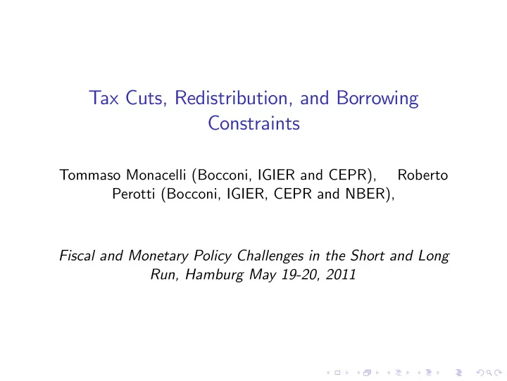
Tax Cuts, Redistribution, and Borrowing Constraints Tommaso Monacelli (Bocconi, IGIER and CEPR), Roberto Perotti (Bocconi, IGIER, CEPR and NBER), Fiscal and Monetary Policy Challenges in the Short and Long Run, Hamburg May 19-20, 2011

Recent debate on the …scal stimulus I Higher spending vs. lower taxes I Tax changes: pro- poor or pro- rich ?

Conventional wisdom 1. Lower taxes better because no implementation lags 2. But e¤ect on private spending can be minimal if households decide to save 3. In a recession, should redistribute in favor of low-income agents, because higher MPC

MPC higher for low income agents: evidence I MPC out of transitory income shocks (Parker 1999, McCarthy 1995, Dynan, Skinner and Zeldes 2001) I Tax rebates (Parker 1999, Souleles 1999, Shapiro and Slemrod 2003, Johnson, Parker and Souleles 2006).

More general questions 1. What are the aggregate e¤ects of redistributing income? 2. Are e¤ects of progressive tax cuts di¤erent from e¤ects of regressive cuts? I Rarely addressed in a general equilibrium macroeconomic model

Tax redistributions: a …rst look at the data I Each US tax bill since 1945 I Assemble data on the level and composition of four categories of taxes 1. personal income taxes 2. corporate income taxes 3. indirect taxes 4. social security taxes

Distributional impact of Personal Income Taxes 1. Employ original documentation by the Joint Committee of Taxation 2. Provide narrative estimate of how each tax bill impacts on the taxes paid by individuals in each income bracket 3. Data on the IRS Statistics on Income ! estimate the number of individuals in each tax bracket, and the total income in each tax bracket.

I Measure how much of the total change in taxes from a given tax bill will be borne by each decile or quartile of income.

Reagan 1981 Tax Cut

Clinton 1993 Tax Increase

Bush 2001 Tax Cut

Bush 2003 Tax Cut

"Poor-biased" tax change I The …rst two quartiles pay more than 50 percent of the increase in taxes (or bene…t for more than 50 percent of the decline in taxes).

Some theory

Our approach 1. Heterogenous agents: patient vs. impatient 2. Impatient agents face borrowing limit (as in classic Bewley-Ayiagary-Hugget) 3. Impatience motivates borrowing ( not idiosyncratic shocks)

Results 1. If prices ‡exible ! redistribution neutral or contractionary 2. If prices sticky ! redistribution (largely) expansionary I Address role of borrowing constraints, nominal rigidities, persistence, govt. debt

Model: households ( ) ∞ β t ∑ max E 0 j [ u ( c j , t ) � v ( n j , t )] j = b , s t = 0 β s > β b |{z} |{z} savers borrowers c j , t + r t � 1 d j , t � 1 = d j , t + w t n j , t � τ j , t + σ j P t |{z} |{z} lump-sum pro…ts share d b , t � d | {z } borrowing constraint

E¢ciency conditions 0 ( n j , t ) v = w t cons/leisure λ j , t λ s , t = β s r t E t f λ s , t + 1 g Euler for savers λ b , t = β b r t E t f λ b , t + 1 g + λ b , t ψ t Pseudo-Euler for borrowers |{z} shadow value of borrowing

Notice 1. If borrowing constraint binding ψ t > 0 ! λ b , t > λ s , t | {z } borrowers have higher shadow value of wealth 2. Credit premium � � r t λ b , t = β b E t f λ b , t + 1 g 1 � ψ t

Firms I Perfect competition ! ∑ y t = F ( n t ) = F n j , t | {z } j production function 0 ( n t ) = 1 w t = F | {z } if CRS

Government ∑ τ j , t = g |{z} j …xed govt. spending

Neutrality 1. Perfect competition 2. Constant return to scale (CRS) 3. Steady state taxes are the same across agents 4. d = 0 0 ( n t ) n s , t c s , t + τ s , t � ( r t � 1 � 1 ) d = F | {z } zero 0 ( n t ) n b , t c b , t + τ b , t + ( r t � 1 � 1 ) d = F | {z } zero c s , t n ϕ 0 ( n t ) s , t = F c b , t n ϕ 0 ( n t ) b , t = F

More generally I d > 0 I DRS or monopolistic competition ! Equilibrium pro…ts deviate from zero I Natural assumption: savers hold shares of …rms ! Result : redistribution pro-borrowers is contractionary

Redistribution from Savers to Borrowers: Flex Prices and Decreasing Returns Output 0 -0.05 -0.1 -0.15 -0.2 0 2 4 6 8 10 12 14 Aggregate Consumption 0 -0.05 -0.1 -0.15 -0.2 0 2 4 6 8 10 12 14

Intuition for contraction: asymmetry index I Endowment economy ! Each agent receive y t / 2 in every period I Resource constraint must imply ! � c s � � c b � b y t = b c s , t + b c b , t y y � c s � b y t b b c b , t = ( c b / y ) � c s , t c b | {z } asymmetry index c s > c b | {z } steady state

I If savers ’ ss consumption larger j ∆ b c b , t j > j ∆ b c s , t j j ∆ b | {z } j borrowers’ n b , t > j ∆ b | {z } j savers’ n s , t l.supply l.supply falls rises I Asymmetric wealth e¤ect on labor supply

Nominal rigidities I New Keynesian setup + heterogenous agents + borrowing constraint I Model inherently dynamic I Role of borrowing constraints in intertemporal substitution

Nominal rigidities � Z 1 � ε / ( ε � 1 ) 0 y t ( i ) ( ε � 1 ) / ε di y t = …nal good y t ( i ) = n t ( i ) i 2 [ 0 , 1 ] pf. di¤erentiated varieties ( 1 + i t ) = r π φ π monetary policy t

Nominal rigidities I Suppose prices …xed for two periods (t and t+1) ! Riskless real int. rate constant I Savers’ Euler equation implies c s , t = c s , t � 1 = c s |{z} savers’ consumption constant I Borrowers’ consumption not constant � c b , t � r β b E t = 1 � ψ t |{z} c b , t + 1 | {z } constant movements riskless in credit rate premium

Nominal rigidities y t = g + c s + c b , t |{z} B.consumption drives aggr. output

Tax redistribution ∆ τ s , t = � ∆ τ b , t > 0 I Transmission # τ b , t ! # ψ t ! " c b , t ! " y t |{z} |{z} output credit premium expansion

Labor market I Aggregate labor supply � � � � c j , t , w t c b , t , c s , w t n t = ∑ n j , t = ∑ l � L p t p j j I Aggregate labor demand � w t µ t � n t = N p

Labor market Aggregate labor market e¤ects of a pro-borrower tax redistribution under rigid prices.

Staggered prices

Output 0.4 0.3 0.2 0.1 0 0 1 2 3 4 5 6 7 8 9 10 Aggregate Consumption 0.4 0.3 0.2 0.1 0 0 1 2 3 4 5 6 7 8 9 10 Aggregate e¤ects of a pro-borrower tax redistribution: staggered prices.

Responses to a Tax Redistribution from Savers to Borrowers Consumption Hours 2 2 savers borrowers 1 1 0 0 -1 -1 0 5 10 0 5 10 Finance Premium Real Riskless Rate 0 0.4 -0.2 0.3 -0.4 0.2 -0.6 0.1 -0.8 0 0 5 10 0 5 10 Responses to a tax redistribution from the savers to the borrowers: sticky prices.

Temporary vs. Permanent Redistributions Output Multiplier 4.5 4 3.5 3 2.5 2 1.5 1 0.5 0 -0.5 0 0.1 0.2 0.3 0.4 0.5 0.6 0.7 0.8 0.9 1 persistence in tax shock Aggregate output impact multiplier of a tax redistribution that favors the borrowers.

Extensions 1. Endogenous borrowing limit 2. Government debt

Endogenous borrowing limit d b , t � ( 1 � χ ) E t f w t + 1 n b , t + 1 g r t | {z } can collateralize a fraction of future L. income

Government debt Savers Fin. Intermediaries Borrowers s t = d b , t + ∆ ( d b , t ) govt. bonds B t d b , t � d b | {z } intermed. frictions ( 1 + i d t ) riskless deposits s t ( 1 + i t ) = ( 1 + δ t ) | {z } spread

Debt-…nanced redistributions g t + ( 1 + i t � 1 ) B t � 1 = B t + ∑ τ j , t govt. budget constraint π t j = s , b τ j , t = ( 1 � ρ τ ) τ j + ρ τ τ j , t � 1 + φ B j B t � 1 + ε j , t | {z } reaction to govt. debt

Sharing the burden of debt stabilization φ B φ B b = 0 s > 0 only savers’ taxes adjust φ B φ B b > 0 s > 0 both taxes adjust

Debt-…nanced redistribution

Flexible prices Aggregate Output 0.02 φ b = 0 0.015 φ b = 0.05 φ b = 0.1 0.01 φ b = 0.5 0.005 0 -0.005 -0.01 0 2 4 6 8 10 12 14 Aggregate Consumption 0.02 0.015 0.01 0.005 0 -0.005 -0.01 0 2 4 6 8 10 12 14 A tax cut to the borrowers under alternative values of φ B b : ‡exible prices.

Sticky prices Aggregate Output 1.5 φ b = 0 1 φ b = 0.05 φ b = 0.1 0.5 φ b = 0.5 0 -0.5 0 2 4 6 8 10 12 14 Aggregate Consumption 1.5 1 0.5 0 -0.5 0 2 4 6 8 10 12 14 A tax cut to the borrowers under alternative values of φ B b : sticky prices.