T HE PERMUTATION MODEL G ( n , 2 d ) 1 , . . . , d iid uniform - PowerPoint PPT Presentation
S PECTRAL DYNAMICS OF RANDOM REGULAR GRAPHS AND THE P OISSON FREE FIELD Soumik Pal The Pitman conference June 21, 2014 G RAPHS AND ADJACENCY MATRICES 3 2 Undirected graphs on n labeled vertices. 4 1 Regular: degree d . 5 6 Adjacency
S PECTRAL DYNAMICS OF RANDOM REGULAR GRAPHS AND THE P OISSON FREE FIELD Soumik Pal The Pitman conference June 21, 2014
G RAPHS AND ADJACENCY MATRICES 3 2 Undirected graphs on n labeled vertices. 4 1 Regular: degree d . 5 6 Adjacency matrix = n × n 0 1 0 0 1 1 symmetric matrix. 1 0 0 1 1 0 0 0 0 1 1 1 Sparse - d ≪ n . 0 1 1 0 0 1 1 1 1 0 0 0 1 0 1 1 0 0
M ODELS OF RANDOM REGULAR GRAPHS The permutation model: G ( n , 2 ) . π - random permutation on [ n ] . 2-regular graph: 3 9 4 8 2 1 7 10 6 5
T HE PERMUTATION MODEL G ( n , 2 d ) π 1 , . . . , π d iid uniform permutations. Superimpose.
T HE PERMUTATION MODEL G ( n , 2 d ) π 1 , . . . , π d iid uniform permutations. Superimpose. 4 3 π 1 = 5 2 π 2 = 1
T HE PERMUTATION MODEL G ( n , 2 d ) π 1 , . . . , π d iid uniform permutations. Superimpose. 4 3 π 1 = ( 1 3 2 )( 4 5 ) 5 2 π 2 = 1
T HE PERMUTATION MODEL G ( n , 2 d ) π 1 , . . . , π d iid uniform permutations. Superimpose. 4 3 π 1 = ( 1 3 2 )( 4 5 ) 5 2 π 2 = ( 1 4 2 ) 1
T HE PERMUTATION MODEL G ( n , 2 d ) π 1 , . . . , π d iid uniform permutations. Superimpose. 4 3 π 1 = ( 1 3 2 )( 4 5 ) 5 2 π 2 = ( 1 4 2 ) 1 Multiple edges, loops OK.
R ANDOM M ATRIX T HEORY A GOE is a square random matrix with
R ANDOM M ATRIX T HEORY A GOE is a square random matrix with − 0 . 6 0 . 7 0 . 1 0 . 3 2 . 1 2 . 5 − 0 . 1 upper triangular entries − 2 . 2 1 . 1 chosen iid N ( 0 , 1 ) ; 0 . 4 A sample of a 4 × 4 GOE matrix and its 3 × 3 minor.
R ANDOM M ATRIX T HEORY A GOE is a square random matrix with − 0 . 6 0 . 7 0 . 1 0 . 3 0 . 7 2 . 1 2 . 5 − 0 . 1 upper triangular entries 0 . 1 2 . 5 − 2 . 2 1 . 1 chosen iid N ( 0 , 1 ) ; 0 . 3 − 0 . 1 1 . 1 0 . 4 symmetric. A sample of a 4 × 4 GOE matrix and its 3 × 3 minor.
R ANDOM M ATRIX T HEORY A GOE is a square random matrix with − 0 . 6 0 . 7 0 . 1 0 . 3 0 . 7 2 . 1 2 . 5 − 0 . 1 upper triangular entries 0 . 1 2 . 5 − 2 . 2 1 . 1 chosen iid N ( 0 , 1 ) ; 0 . 3 − 0 . 1 1 . 1 0 . 4 symmetric. Minor=principal submatrix, A sample of a 4 × 4 GOE matrix also GOE. and its 3 × 3 minor.
GOE VS . RANDOM GRAPHS Adjacency matrices are not GOE (or, Wigner). Rows are sparse; no independence.
GOE VS . RANDOM GRAPHS Adjacency matrices are not GOE (or, Wigner). Rows are sparse; no independence. However, for large d , approximately GOE. Eigenvalue distribution (McKay ’81, Dumitriu-P . ’10, Tran-Vu-Wang ’10) Linear eigenvalue statistics (Dumitriu-Johnson-P .-Paquette ’11) Simulations. Not Erd˝ os-Rényi, e.g. connected.
E IGENVALUE FLUCTUATIONS W ∞ - GOE array. W n - n × n minor. E-values { λ n i } . Linear eigenvalue statistics � λ n n � � i 2 √ n tr f ( W n ) := f . i = 1 (Classical Theorem) If f is analytic 0 , σ 2 � � n →∞ [ tr f ( W n ) − E tr f ( W n )] = N lim . f
D YNAMICS OF EIGENVALUE FLUCTUATIONS (A. Borodin ’10) GOE array W ∞ ( s ) in time with entries as Brownian motions. Choose ( t i , s i , f i , i = 1 , . . . , k ) . Polynomial f i ’s. � � � � lim tr f i W ⌊ nt i ⌋ ( s i ) − E tr f i ( · ) , i ∈ [ k ] = Gaussian . n →∞ Mean zero. Covariance kernel?
D YNAMICS OF EIGENVALUE FLUCTUATIONS (A. Borodin ’10) GOE array W ∞ ( s ) in time with entries as Brownian motions. Choose ( t i , s i , f i , i = 1 , . . . , k ) . Polynomial f i ’s. � � � � lim tr f i W ⌊ nt i ⌋ ( s i ) − E tr f i ( · ) , i ∈ [ k ] = Gaussian . n →∞ Mean zero. Covariance kernel? Fix s . Limiting Height Function is the Gaussian Free Field. Nontrivial correlation across s .
M AIN QUESTION What dynamics on random regular graphs leads to similar eigenvalue fluctuations in dimension × time?
Description of the dynamics
D YNAMICS IN DIMENSION (Dubins-Pitman) Chinese restaurant process on d permutations. i th customers arrive simultaneously. Sits independently. Let T i = Exp( i ), i ∈ N , � m � � n t = max m : T i ≤ t . i = 1 G ( t , 0 ) := G ( n t , 2 d ) , for 0 ≤ t ≤ T . dimension t ; time 0.
D YNAMICS IN TIME Fix T large. d permutations on n labels. Run random transposition MC simultaneously. � n � Any transposition selected at rate 1 / n . 2 Successive product on left. Superimpose - G ( T , s ) for s ≥ 0. Delete labels successively: G ( T + t , s ) , t ∈ [ − T , 0 ] , s ≥ 0 .
C YCLES AND EIGENVALUES N k - # k -cycles in the graph G ( n , 2 d ) . As n → ∞ , ( N k , k ∈ N ) - linear eigenvalue statistics. In fact 2 kN k ≈ tr ( T k ( G ( n , 2 d ))) . ( T k , k ∈ N ) - Chebyshev polynomials of first kind.
Dynamics of cycles in dimension
G ROWTH OF A CYCLE (Johnson-P . ’12) Existing cycles grow in size. 4 π 2 3 4 π 2 3 π 1 6 π 1 π 1 π 1 π 1 5 2 5 2 π 2 π 1 π 2 π 1 1 1 π 1 = ( 1 2 3 )( 4 5 ) π 1 = ( 1 2 6 3 )( 4 5 ) π 2 = ( 1 5 )( 4 3 )( 2 ) π 2 = ( 1 5 )( 4 3 )( 2 6 ) F IGURE : Vertex 6 is inserted between 2 and 3 in π 1 .
B IRTH OF A CYCLE 6 π 1 π 2 π 2 π 1 π 2 π 1 π 2 π 3 π 2 π 1 1 2 3 4 5 1 2 3 4 5 π 1 = ( 2 3 1 )( 4 5 ) π 1 = ( 2 3 1 6 )( 4 5 ) π 2 = ( 2 1 3 4 5 ) π 2 = ( 2 1 3 4 6 5 ) F IGURE : A cycle forms “spontaneously”.
C YCLE COUNTS C ( T ) ( t ) = # k -cycles in G ( T + t , 0 ) , t ∈ [ − T , 0 ] . k Non-Markovian process in t , with T fixed.
C YCLE COUNTS C ( T ) ( t ) = # k -cycles in G ( T + t , 0 ) , t ∈ [ − T , 0 ] . k Non-Markovian process in t , with T fixed. ( C ( T ) ( t ) , k ∈ N , t < 0 ) converges as T → ∞ . k Limiting process ( N k ( t ) , k ∈ N , t ≤ 0 ) is Markov. Running in stationarity.
T HE LIMITING PROCESS (Johnson-P . ’12) In the limit: Existing k -cycles grows to ( k + 1 ) at rate k . New k -cycles created at rate µ ( k ) ⊗ Leb. Here: µ ( k ) = 1 2 [ a ( d , k ) − a ( d , k − 1 )] , k ∈ N , a ( d , 0 ) := 0 , where � ( 2 d − 1 ) k − 1 + 2 d , k even , a ( d , k ) = ( 2 d − 1 ) k + 1 , k odd .
P OISSON FIELD OF Y ULE PROCESSES k x x x Poisson point process χ on N × ( −∞ , ∞ ) . Intensity µ ⊗ Leb.
P OISSON FIELD OF Y ULE PROCESSES k x x x Poisson point process χ on N × ( −∞ , ∞ ) . Intensity µ ⊗ Leb. For ( k , y ) ∈ χ , start indep Yule processes ( X k , y ( t ) , t ≥ 0 ) .
P OISSON FIELD OF Y ULE PROCESSES k x x x Poisson point process χ on N × ( −∞ , ∞ ) . Intensity µ ⊗ Leb. For ( k , y ) ∈ χ , start indep Yule processes ( X k , y ( t ) , t ≥ 0 ) . Define � N k ( t ) := 1 { X j , y ( t − y ) = k } . ( j , y ) ∈ χ ∩{ [ k ] × ( −∞ , t ] }
I NVARIANT DISTRIBUTION � � C ( T ) ( t ) , k ∈ N , t ∈ ( −∞ , 0 ] − → ( N k ( t ) , k ∈ N , t ∈ ( −∞ , 0 ]) . k Marginal distribution: � a ( d , k ) � ( N k ( t ) , k ∈ N ) ∼ ⊗ Poi . 2 k
I NVARIANT DISTRIBUTION � � C ( T ) ( t ) , k ∈ N , t ∈ ( −∞ , 0 ] − → ( N k ( t ) , k ∈ N , t ∈ ( −∞ , 0 ]) . k Marginal distribution: � a ( d , k ) � ( N k ( t ) , k ∈ N ) ∼ ⊗ Poi . 2 k Dumitriu-Johnson-P .-Paquette ’11 Bollobás ’80, Wormald ’81.
C YCLES IN TIME j 1 1 6 2 6 2 5 3 5 3 4 4 F IGURE : A cycle that vanishes due to transposition ( 1 , j ) , j > 6. Random transpositions make short cycles vanish or appear at random. Other effects are of negligible probability.
T HE JOINT LIMITING PROCESS (Ganguly-P . ’14) Take limit as T → ∞ . Fix t < 0. Consider in s ≥ 0. ( N k ( t , · ) , k ∈ N ) - independent birth-and-death chains. Joint convergence to a Poisson surface: � � C ( T ) ( t , s ) , k ∈ N , t ≤ 0 , s ≥ 0 − → ( N k ( t , s )) . k Yule process in dimension, birth-and-death chains in time. Markov field. Stationary along axis. Joint law by intertwining.
Diffusion limit
L ARGE DIMENSION , SMALL TIME Take centered+scaling limit as d → ∞ and s = ve − T 0 , t = − T 0 + u , T 0 → ∞ , u ≥ 0 , v ≥ 0 . Large dimension; very small time. Imagine observing random transposition chain acting on infinite symmetric group.
O RNSTEIN -U HLENBECK T HEOREM (J OHNSON -P. ’12, G ANGULY -P. ’14) Joint convergence to Gaussian field: ( 2 d − 1 ) − k / 2 � 2 kN k ( − T 0 + u , ve − T 0 ) − E ( · ) � − → ( U k ( u , v )) . U k ( · , · ) - continuous Gaussian surfaces, independent among k. Infinite-dimensional O-U surface. Marginally N ( 0 , k / 2 ) . In dimension and time ( U k ) time-changed stationary O-U: dU k ( t , · ) = − kU k ( t , · ) dt + kdW k ( t ) , t ≥ 0 .
C OMPARISON WITH W IGNER Recall 2 kN k ≈ tr ( T k ( · )) . Allows to compute covariances of polynomials linear eigenvalue statistics. Same as GOE. A diffusion dynamics on the Gaussian Free Field.
Thank you Jim for all the beautiful math and happy birthday.
Recommend
More recommend
Explore More Topics
Stay informed with curated content and fresh updates.
