Stokes waves with constant vorticity: Numerical computation Vera - PowerPoint PPT Presentation

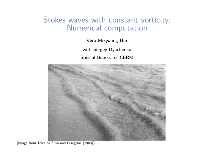
Stokes waves with constant vorticity: Numerical computation Vera Mikyoung Hur with Sergey Dyachenko F . Trlrs do, Silva (md I ) . 298 A . 11. Peregrine Special thanks to ICERM (Image from Teles da Silva and Peregrine (1988)) FICCKE 1.5. X surfwe shear wavr occurring naturally in backwash on a beach. described in Peregrine (1974). That model was stimulated by the observation of steep large rounded waves in the backwash of waves incident on beaches. Such a wave arising naturally is shown in the photograph of figure 15. Another surface shear wave also described in Peregrine (1974) is the ‘wave hydraulic jump’ (see also discussion of that paper). Both of these waves are easily reproduced in the laboratory, and are usually almost stationary on a fast moving strcam. They occur over fixed beds. but also seem to have a counterpart in supercritical flow over antidunes on a mobile bed. Peregrine’s (1974) model does not depend on a specific vorticity distribution but simply characterizes the thin sheet of surface water by its momentum flux and considers its deflection due to hydrostatic pressure in the almost stagnant water beneath it. The ordinary differential equation so obtained for the shape of the wave is the same as that for the finite bending of a thin beam or elastiea. This gives an easy way of comparing Peregrine‘s solution with the figures in this paper : just take a piece of paper or card and bend it whilst holding it at each side. Comparison with figure 14 will show that most of the wave closely follows such a curve. The pressurc field in figure 14(b) is easily interpreted in terms of a high-speed surface flow. A high transverse pressure gradient is required to turn the flow sharply at the bast of the wave, hence the substantial excess pressures on the bed. Then over the main portion of the wave the pressure falls below atmospheric as in Peregrine’s (1974) model, and ‘sucks’ the surface jet around in a curve which is tighter than the corresponding free-fall parabola. As the jet ‘lands’ near the bed once again high pressure gradients turn it back into a horizontal flow. To some extent the constant vortieity flow here may be a better model than Peregrine’s for very steep waves over closed eddies. This is due to the Prandtl-Batchelor result that in two-dimensional high-Reynolds-number flow steady recirculating regions with closed streamlines have constant vorticity. /�����3�7��8B���:DDAC����� 53�4B��97 �B9�5�B7 ��B����2���7BC�D��0�4B3B���������,AB������3D�����������C�4�75D�D��D:7�.3�4B��97�.�B7�D7B�C��8��C7��3�3��34�7�3D :DDAC����� 53�4B��97 �B9�5�B7�D7B�C �:DDAC������ �B9��� �����1����������������

Stokes waves are • traveling waves • periodic • at the surface of an incompressible inviscid fluid = water • two dimensional • acted on by gravity (no surface tension) • infinitely deep or with a rigid flat bed

4/23/2017 1280px-Stokes_wave_max_height.svg.png (1280×310) In the irrotational setting Stokes conjectured (Image from Wikipedia) Amick, Fraenkel, and Toland (1982) proved that such a corner wave exists. Recently, further advances — analytical and numerical — based on Babenko’s equation: https://upload.wikimedia.org/wikipedia/commons/thumb/a/a5/Stokes_wave_max_height.svg/1280px-Stokes_wave_max_height.svg.png 1/1 λ 2 H y 1 “ y ` y H y 1 ` H p yy 1 q , y “ fluid surface, λ “ Froude number, H “ Hilbert transform.

In the rotational setting Constantin and Strauss (2004) worked out global bifurcation for general vorticities. Solutions do not permit critical layers, or internal stagnation. Wahl´ en (2009) observed them for constant vorticities.

For constant vorticities Constantin, Strauss, and Varvaruca (2014) worked out global bifurcation, permitting overhanging, critical layers, and internal stagnation. They conjectured that the limiting wave is: or By the way, the proof is non -constructive. Our goal is to numerically study the conjecture.

Earlier works include • Simmen and Saffman (1985), • Teles da Silva and Peregrine (1988), • Vanden-Broeck (1994, 1996), .... See also • Vasan and Oliveras (2014), • Ribeiro, Milewski, and Nachbin (2017),...

E’. Teles da Silva and D. H . 284 A , Peregrine Formulation E’. Teles da Silva and D. H . 284 A , Peregrine downstream “ ´ vorticity upstream “ ` vorticity FIGURE 1. Sketches indicating wave direction and shear profile. On the left (i) is the configuration we use, and on the right (ii) the equivalent wave stationary on a stream. (a) Wave propagating (Figures from Teles da Silva and Peregrine (1983)) upstream, positive vorticity. (b) Wave propagating downstream, negative vorticity. Let’s write the velocity p´ ωy ´ c, 0 q ` ∇ φ , Using (2.9) and comparing with the undisturbed flow we can interpret (2.10) as ω “ constant vorticity, c “ wave speed. showing that the waves travel symmetrically with respect to thc flow at a depth c : tanh (kh) W = - = The problem is written: (2.11) 29 FIGURE 1. Sketches indicating wave direction and shear profile. On the left (i) is the configuration 2k ’ we use, and on the right (ii) the equivalent wave stationary on a stream. (a) Wave propagating ∆ φ “ 0 in fluid, upstream, positive vorticity. (b) which gives a measure of the depth of water which influences the wave properties, or Wave propagating downstream, negative vorticity. 2 ωy 2 ´ cy “ 0 ‘wave depth’. The limiting values of W for large and small kh are 6k-’ and ih ψ ´ 1 at surface, respectively. The right-hand side of (2.10) shows that shear increases the wave speed 2 p φ x ´ ωy ´ c q 2 ` 1 1 2 φ 2 y ` gy “ B at surface, of linearized waves. Using (2.9) and comparing with the undisturbed flow we can interpret (2.10) as φ y “ 0 at bed, A critical layer occurs in the flow if at any depth showing that the waves travel symmetrically with respect to thc flow at a depth ψ “ harmonic conjugate of φ , B “ Bernoulli constant. -5Y, c = c : tanh (kh) W = - = (2.11) 29 let h, = 2k ’ c / < be the critical layer depth. Substitution in the linear dispersion equation (2.8) and use of the wave depth, W , gives which gives a measure of the depth of water which influences the wave properties, or ‘wave depth’. The limiting values of W for large and small kh are 6k-’ and ih h, = W+W(l+&), respectively. The right-hand side of (2.10) shows that shear increases the wave speed of linearized waves. for linear waves. A critical layer occurs in the flow if at any depth Thus if then: is a critical layer it is always at a depth greater than 2W, and then only ncar 2W for strong shcars. Critical laycrs only occur for waves propagating -5Y, c = ‘ upstream ’, and when let h, = c / < be the critical layer depth. Substitution in the linear dispersion equation (2.12) (2.8) and use of the wave depth, W , gives In order to fix ideas we shall only consider positive values of c and k but allow 5 h, = W+W(l+&), to have either sign. For convenience of description we shall refer to ‘upstream’ and ‘downstream ’ in the sense of waves propagating on a flowing stream with maximum for linear waves. in which our configuration for 5 positive is velocity at the surface. See figure 1 Thus if then: is a critical layer it is always at a depth greater than 2W, and then (a) shown and tho effect of a stream giving wave propagation ‘upstream’. Similarly only ncar 2W for strong shcars. Critical laycrs only occur for waves propagating shows 5 negative and the corresponding ‘downstream’ figure l(6) propagation. The upstream ’, and when ‘ downstream case is equivalent to downwind propagation for the case of a shear (2.12) generated by the wind. In order to fix ideas we shall only consider positive values of c and k but allow 5 to have either sign. For convenience of description we shall refer to ‘upstream’ and ‘downstream ’ in the sense of waves propagating on a flowing stream with maximum /�����3�7��8B���:DDAC����� 53�4B��97 �B9�5�B7 ��B����2���7BC�D��0�4B3B���������,AB������3D�����������C�4�75D�D��D:7�.3�4B��97�.�B7�D7B�C��8��C7��3�3��34�7�3D :DDAC����� 53�4B��97 �B9�5�B7�D7B�C �:DDAC������ �B9��� �����1���������������� in which our configuration for 5 positive is velocity at the surface. See figure 1 (a) shown and tho effect of a stream giving wave propagation ‘upstream’. Similarly shows 5 negative and the corresponding ‘downstream’ figure l(6) propagation. The downstream case is equivalent to downwind propagation for the case of a shear generated by the wind. /�����3�7��8B���:DDAC����� 53�4B��97 �B9�5�B7 ��B����2���7BC�D��0�4B3B���������,AB������3D�����������C�4�75D�D��D:7�.3�4B��97�.�B7�D7B�C��8��C7��3�3��34�7�3D :DDAC����� 53�4B��97 �B9�5�B7�D7B�C �:DDAC������ �B9��� �����1����������������