Statistical methods in bioinformatics Integrative data analysis - PowerPoint PPT Presentation

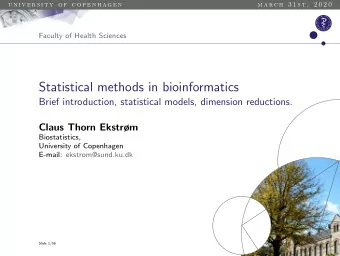
u n i v e r s i t y o f c o p e n h a g e n a p r . 3 r d , 2 0 2 0 Faculty of Health Sciences Statistical methods in bioinformatics Integrative data analysis Claus Thorn Ekstrøm Biostatistics, University of Copenhagen E-mail: ekstrom@sund.ku.dk Slide 1/57

u n i v e r s i t y o f c o p e n h a g e n a p r . 3 r d , 2 0 2 0 Summary so far So far we have mainly considered two situations: 1 Large number of outcomes, few predictors. 2 One outcome, large number of predictors. • GWAS, gene expression, lasso, pca, ... • For example: Networks, (could swap outcome/predictors), ... Slide 2/57 — Statistical methods in bioinformatics

u n i v e r s i t y o f c o p e n h a g e n a p r . 3 r d , 2 0 2 0 Summary so far • General techniques • Networks and text mining • GWAS and genomics • RNA Slide 3/57 — Statistical methods in bioinformatics

u n i v e r s i t y o f c o p e n h a g e n a p r . 3 r d , 2 0 2 0 The omics revolution Slide 4/57 — Statistical methods in bioinformatics

u n i v e r s i t y o f c o p e n h a g e n a p r . 3 r d , 2 0 2 0 Revisiting correlation The Pearson correlation between to quantitative variables, X , and Y is ∑ n i =1 ( x i − ¯ x )( y i − ¯ y ) ˆ ρ = � ( ∑ n x ) 2 )( ∑ n y ) 2 ) i =1 ( x i − ¯ i =1 ( y i − ¯ Measures the linear relationship between X and Y . Slide 5/57 — Statistical methods in bioinformatics

u n i v e r s i t y o f c o p e n h a g e n a p r . 3 r d , 2 0 2 0 Revisiting correlation Slide 6/57 — Statistical methods in bioinformatics

u n i v e r s i t y o f c o p e n h a g e n a p r . 3 r d , 2 0 2 0 Next generation correlation = MIC ? Can we do something more advanced than simple correlations? Maximum information correlation Slide 7/57 — Statistical methods in bioinformatics

u n i v e r s i t y o f c o p e n h a g e n a p r . 3 r d , 2 0 2 0 Next generation correlation = MIC ? Can we do something more advanced than simple correlations? Maximum information correlation Slide 7/57 — Statistical methods in bioinformatics

u n i v e r s i t y o f c o p e n h a g e n a p r . 3 r d , 2 0 2 0 Example — from MIC paper Slide 8/57 — Statistical methods in bioinformatics

u n i v e r s i t y o f c o p e n h a g e n a p r . 3 r d , 2 0 2 0 dCor — distance correlation matrix Produces a measure of variable dependence: From 0 (corresponds to statistical independence) to 1 (no noise). • Produces number between 0 and 1 • Can have different dimensions (but requires same N ) • Can detect both linear and non-linear dependence • Approximates standard Pearson correlation coefficient when relationship is roughly linear. Slide 9/57 — Statistical methods in bioinformatics

u n i v e r s i t y o f c o p e n h a g e n a p r . 3 r d , 2 0 2 0 dCor > library("energy") # Pearson cor: -0.068 > cor(x,y); dcor(x, y) # dcor = 0.2291 ● ● ● ● ● ● ● ● ● ● ● ● ●● ● ● ● ● ● ● ● ● ● ● ● ● ● ● ● ● ● ●● ● ● ● ● ● ● ● ● ● ● ● ● ● ● ● ● ● ● 70 ● ● ● ● ● ● ● ● ● ● ● ● ● ● ● ● ● ● ● ● y ● 50 ● ● ● ● ● ● ● ● ● ● 30 ● ● ● ● ● ● ● ● ● ● ● ● ● ● ● ● ● ● ● ● ● ● ● ● ●● ● ● ● ● ● ● ● ● ● ● ● ● ● ● ● ● ● ● ● ● ● ● ● ● ● ● ● ● ● ● ● ● ● ● Slide 10/57 — Statistical methods in bioinformatics

u n i v e r s i t y o f c o p e n h a g e n a p r . 3 r d , 2 0 2 0 Computing dCor Compute the distance correlation between X ∈ R N k and Y ∈ R N j . 1 Compute matrix of Euclidian distances between N cases for X and Y . 2 Perform double centering for each matrix 3 Multiply the matrices element-wise and compute sum. 4 Divide by N 2 (ie, compute average). 5 Take square root. This is the distance covariance. 6 Variances can be computed for each matrix against itself. 7 The distance correlation is computed similarly to the Pearson correlation. Slide 11/57 — Statistical methods in bioinformatics

u n i v e r s i t y o f c o p e n h a g e n a p r . 3 r d , 2 0 2 0 Computing dCor ( X , Y ) = [(0 , 0) , (0 , 1) , (1 , 0) , (1 , 1)] Slide 12/57 — Statistical methods in bioinformatics

u n i v e r s i t y o f c o p e n h a g e n a p r . 3 r d , 2 0 2 0 Inference What about inference? For a given pair of high-dimensional variables: • Compute a modified version of the distance correlation. • Use dcov.ttest() Slide 13/57 — Statistical methods in bioinformatics

u n i v e r s i t y o f c o p e n h a g e n a p r . 3 r d , 2 0 2 0 NGS / RNA-seq Microarrays are limited in what we can find as we can only measure intensities of the probes already on the array. High-throughput DNA sequencing methods / next-generation sequencing Slide 14/57 — Statistical methods in bioinformatics

u n i v e r s i t y o f c o p e n h a g e n a p r . 3 r d , 2 0 2 0 Gene variant calling Slide 15/57 — Statistical methods in bioinformatics

u n i v e r s i t y o f c o p e n h a g e n a p r . 3 r d , 2 0 2 0 NGS technologies Recall from this Monday: 1 Align sequenced fragments with reference sequence (alternatively make de novo assembly). • really a non-trivial task, but will not go into details. abundance. 2 Count the number of fragments mapping to certain regions • usually, genes • The read counts linearly approximate target transcript abundance. A large number of short DNA fragments. The reads are then used for several applications, e.g., sequence reconstruction, DNA assembly, gene expression profiling, mutation analysis. Slide 16/57 — Statistical methods in bioinformatics

u n i v e r s i t y o f c o p e n h a g e n a p r . 3 r d , 2 0 2 0 Normalization Number of reads are approximately proportional to length of transcript, the total number of mapped reads. Typically considering the reads per kilobase per million reads (RPKM) or variations on this theme. 1 Count up the total reads; divide by 1,000,000 ⇒ “per million”scaling factor. 2 Divide read counts by the“per million”scaling factor to normalize for sequencing depth (RPM) 3 Divide the RPM values by the length of the gene, in kilobases. This gives you RPKM. Slide 17/57 — Statistical methods in bioinformatics

u n i v e r s i t y o f c o p e n h a g e n a p r . 3 r d , 2 0 2 0 Modeling read counts Back to the linear model? count i = X β + ε i Assumption of continuous data each gene. But they really are counts (discrete) and relatively infrequent. Let N i be total number of fragments counted in sample i , and p i the probability that a fragment matches a particular gene of interest. The observed number of reads for gene in sample i is R i ∼ Poisson( N i p i ) Note: E ( R i ) = Var( R i ) = N i p i . Slide 18/57 — Statistical methods in bioinformatics

u n i v e r s i t y o f c o p e n h a g e n a p r . 3 r d , 2 0 2 0 Modeling read counts Wish to, say, compare two groups: cases and controls? Assume log( p i = α + β x i ), where x i is 0 (controls) or 1 (cases). Generalized linear model (Poisson regression): log( E ( R i )) = log( N i ) + α + β x i � �� � Not interesting Hypothesis of no differential expression between the groups H 0 : β = 0 glm(reads ~ group + offset(N), data=DF, family="poisson") Can extend the model to Generalized linear mixed effect (Poisson mixed effect model) to account for additional sources of variation. Slide 19/57 — Statistical methods in bioinformatics

u n i v e r s i t y o f c o p e n h a g e n a p r . 3 r d , 2 0 2 0 Modeling read counts Overdispersion can be a problem. Recall the assumption from the Poisson distribution: E ( R i ) = Var( R i ) = N i p i Slide 20/57 — Statistical methods in bioinformatics

u n i v e r s i t y o f c o p e n h a g e n a p r . 3 r d , 2 0 2 0 Modeling read counts Overdispersion can be a problem. Recall the assumption from the Poisson distribution: E ( R i ) = Var( R i ) = N i p i Alternatives: • Use a Poisson regresion with overdispersion, i.e., where Var( R i ) = σ E ( R i ). • Use another distribution — for example a negative binomial distribution — to describe the read counts. glm(reads ~ group + offset(N), data=DF, family="quasipoisson") Slide 20/57 — Statistical methods in bioinformatics

u n i v e r s i t y o f c o p e n h a g e n a p r . 3 r d , 2 0 2 0 Zero-inflation models The dispersion problem in Poisson/NB models is often caused by zero-inflation. Slide 21/57 — Statistical methods in bioinformatics

u n i v e r s i t y o f c o p e n h a g e n a p r . 3 r d , 2 0 2 0 Zero-inflation models Useful in situations like: • RNA sequence reads • Microbiome data (abundance counts or percentages) • (Some) mixture modeling Slide 22/57 — Statistical methods in bioinformatics

u n i v e r s i t y o f c o p e n h a g e n a p r . 3 r d , 2 0 2 0 Example: microbiome data Slide 23/57 — Statistical methods in bioinformatics