Statistical Inference Definition : A model is a family { P ; } of - PDF document
Statistical Inference Definition : A model is a family { P ; } of possible distributions for some random variable X . WARNING: Data set is X , so X will generally be a big vector or matrix or even more compli- cated object.)
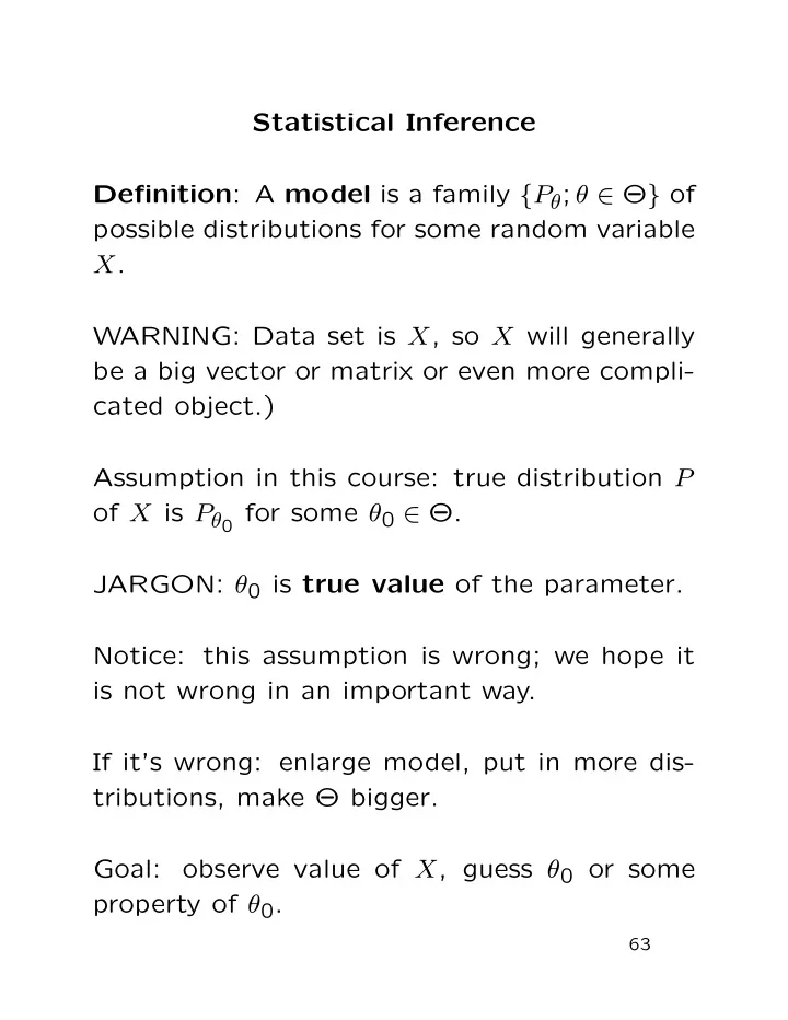
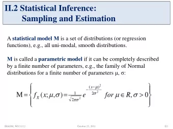
Statistical Inference Definition : A model is a family { P θ ; θ ∈ Θ } of possible distributions for some random variable X . WARNING: Data set is X , so X will generally be a big vector or matrix or even more compli- cated object.) Assumption in this course: true distribution P of X is P θ 0 for some θ 0 ∈ Θ. JARGON: θ 0 is true value of the parameter. Notice: this assumption is wrong; we hope it is not wrong in an important way. If it’s wrong: enlarge model, put in more dis- tributions, make Θ bigger. Goal: observe value of X , guess θ 0 or some property of θ 0 . 63
Classic mathematical versions of guessing: compute estimate ˆ 1. Point estimation: θ = ˆ θ ( X ) which lies in Θ (or something close to Θ). 2. Point estimation of ftn of θ : compute es- timate ˆ φ = ˆ φ ( X ) of φ = g ( θ ). 3. Interval (or set) estimation: compute set C = C ( X ) in Θ which we think will contain θ 0 . 4. Hypothesis testing: choose between θ 0 ∈ Θ 0 and θ 0 �∈ Θ 0 where Θ 0 ⊂ Θ. 5. Prediction: guess value of an observable random variable Y whose distribution de- pends on θ 0 . Typically Y is the value of the variable X in a repetition of the exper- iment. 64
Several schools of statistical thinking. Main schools of thought summarized roughly as fol- lows: • Neyman Pearson : A statistical procedure is evaluated by its long run frequency per- formance. Imagine repeating the data col- lection exercise many times, independently. Quality of procedure measured by its aver- age performance when true distribution of X values is P θ 0 . • Bayes : Treat θ as random just like X . Compute conditional law of unknown quan- tities given knowns. In particular ask how procedure will work on the data we actu- ally got – no averaging over data we might have got. • Likelihood : Try to combine previous 2 by looking only at actual data while trying to avoid treating θ as random. We use Neyman Pearson approach to evaluate quality of likelihood and other methods. 65
Recommend


More recommend
Explore More Topics
Stay informed with curated content and fresh updates.