Statistical Data Mining Definitions Population, Sample, Statistic - PDF document

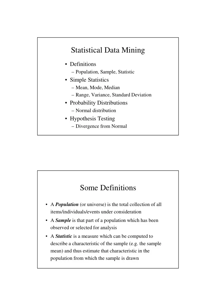
Statistical Data Mining • Definitions – Population, Sample, Statistic • Simple Statistics – Mean, Mode, Median – Range, Variance, Standard Deviation • Probability Distributions – Normal distribution • Hypothesis Testing – Divergence from Normal Some Definitions • A Population (or universe) is the total collection of all items/individuals/events under consideration • A Sample is that part of a population which has been observed or selected for analysis • A Statistic is a measure which can be computed to describe a characteristic of the sample (e.g. the sample mean) and thus estimate that characteristic in the population from which the sample is drawn

Some Simple Statistics The Mean (average) is the sum of the values in a sample divided by the • number of values The Median is the midpoint of the values in a sample (50% above; 50% • below) after they have been ordered (e.g. from the smallest to the largest) The Mode is the value that appears most frequently in a sample • The Range is the difference between the smallest and largest values in a • sample The Variance is a measure of the dispersion of the values in a sample - how • closely the observations cluster around the mean of the sample The Standard Deviation is the square root of the variance of a sample • Moments about the Mean • The m-th moment about the mean of a sample is given by ∑ (X- µ ) m /n • The second moment is the variance • The third moment can be used in tests for skewness • The fourth moment can be used in tests for kurtosis

Probability Distributions • If a population can be shown to conform to a standard probability distribution then a wealth of statistical knowledge and results can be brought to bear on its analysis • On the other hand, if a population is erroneously thought to conform to a particular distribution then the results of the analysis will be flawed • Many standard statistical techniques are based on the assumption that the underlying distribution of a population is Normal (Gaussian) • Statistical tests have been developed to determine whether a sampled population is normally distributed Central Limit Theorem • As more and more samples are taken from a population the distribution of the sample means conforms to a normal distribution • The average of the samples more and more closely approximates the average of the entire population • A very powerful and useful theorem • The normal distribution is such a common and useful distribution that additional statistics have been developed to measure how closely a population conforms to it and to test for divergence from it due to skewness and kurtosis

The Normal (Gaussian) Distribution The Normal distribution is a bell-shaped curve defined by the mean and variance of a population N(0,1) means a normal distribution with mean 0 and variance 1 If a random variable, X, is N( µ , σ 2 ) then the random variable (X- µ )/ σ will be N(0,1) Tests of Normality • There are a number of tests that can be used to check whether a population is normally distributed The χ 2 goodness of fit test is the most popular • • More on this later …

Skewness Sometimes a population is a skewed form of a standard distribution and in such circumstances there exist methods which can be used to take account of this Testing for Skewness • The second and third moments about the mean can be used to test for skewness Coefficient of skewness is denoted by g 1 • g 1 = m 3 /(m 2 √ m 2 )

Kurtosis Kurtosis is a measure of how tall and thin or squashed and fat the bell-shaped curve for a sample is compared to what is required for a normal distribution Testing for Kurtosis • The second and fourth moments about the mean can be used to test for kurtosis • Kurtosis is denoted by g 2 2 ) - 3 g 2 = (m 4 /m 2

Hypothesis Testing I • A statistical hypothesis is a statement about probability distributions • E.g. The observed data is normally distributed • The hypothesis to be tested is called the null hypothesis and commonly denoted by H 0 • The null hypothesis is normally formulated as a statement of “no difference” • E.g. There is no difference between the observed data and that which the normal distribution would suggest • The null hypothesis automatically defines an alternative hypothesis, H 1 , which normally covers all other possibilities (a two-tailed test) • E.g. The observed data is not normally distributed • Sometimes we know that certain situations cannot arise for logical reasons and this might lead us to consider a one-tailed test • E.g. H 0 : A=B and H 1 : A<B because we know B can never be less than A in practice Hypothesis Testing II • A test of a null hypothesis involves determining the likelihood that the data under consideration conform to the hypothesised distribution • E.g. the chi-squared goodness of fit test examines the difference between the observed data and that which would be expected if the data were normally distributed • If the difference is sufficiently small then we can accept the null hypothesis and the magnitude of the difference can give us a measure of how confident we should be in the result • This is the significance level of the test and can be interpreted as the probability that the data would satisfy the hypothesis even if it wasn’t valid • A 5% significance level means a probability of less than 0.05 of this occurring • A 1% significance level means a probability of less than 0.01 of this occurring • Clearly there are two possible types of error that could occur in hypothesis testing • We might reject the null hypothesis when it is, in fact, true (Type I error) • We might accept the null hypothesis when it is, in fact, false (Type II error)

Hypothesis Testing III • If the difference is so large that we do not wish to accept the null hypothesis then we must accept the alternative hypothesis • Note that this leaves us none the wiser as to what the underlying distribution of our data actually is • This probability distribution based approach may seem to impose severe restrictions on the nature of the hypotheses that can be tested statistically but many statements can be re-formulated as statements about probability distributions χ 2 Goodness of fit Test I • This is the classic test of whether a data sample is normally distributed or not • We first group our data into k classes so that we can form a frequency distribution (the number of data items in each class) • We calculate the mean and standard deviation of our sample and define a normal distribution based on these values • We now need to see if the number of data items in each of our classes matches the number predicted by the normal distribution

χ 2 Goodness of fit Test II • For each class we calculate (Observed – Expected) 2 /Expected • We denote Observed by f i and Expected by F i for each class i and then sum the above over all k classes to get χ 2 = ∑ (f i – F i ) 2 /F i This is the χ 2 goodness of fit criterion • • The larger its value the less likely is the hypothesis that our observed values are normally distributed The size of the χ 2 value can be used in conjunction with statistical tables of the χ 2 • distribution (with k-3 degrees of freedom) to determine whether the null hypothesis should be accepted at a given level of significance χ 2 Goodness of fit Test III • Note that even if we can conclude that our data are normally distributed at a very strong level of significance it is still possible that the data might be skewed or contain kurtosis • These should still be tested for