STAT 113: FINAL EXAM PRACTICE PROBLEMS SOLUTIONS Research Design / - - PDF document

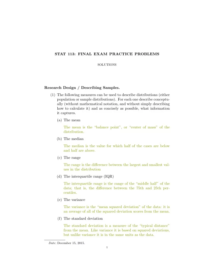
STAT 113: FINAL EXAM PRACTICE PROBLEMS

SOLUTIONS

Research Design / Describing Samples. (1) The following measures can be used to describe distributions (either population or sample distributions). For each one describe conceptu- ally (without mathematical notation, and without simply describing how to calculate it) and as concisely as possible, what information it captures. (a) The mean The mean is the “balance point”, or “center of mass” of the distribution. (b) The median The median is the value for which half of the cases are below and half are above. (c) The range The range is the difference between the largest and smallest val- ues in the distribution (d) The interquartile range (IQR) The interquartile range is the range of the “middle half” of the data; that is, the difference between the 75th and 25th per- centiles. (e) The variance The variance is the “mean squared deviation” of the data: it is an average of all of the squared deviation scores from the mean. (f) The standard deviation The standard deviation is a measure of the “typical distance” from the mean. Like variance it is based on squared deviations, but unlike variance it is in the same units as the data.

Date: December 15, 2015.

1

2 SOLUTIONS

(2) Describe what it means for a measure to be robust/resistant (two terms for the same thing). For each of the measures above, indicate whether it is or is not relatively robust/resitant. What consider- ations go into choosing whether or not to use a robust/resistant measure? A robust/resistant measure is one that cannot be influenced by a small handful of extreme values or outliers. The mean and vari- ance/standard deviation are not robust/resistant, because they are heavily influenced by extreme values/outliers (especially the vari- ance and standard deviation). The range is extremely not robust because it is influenced entirely by extreme observations. The me- dian and interquartile range are considered robust, because they take into account only the values near the middle of the distribution. (3) (Modified/abridged from A.3) In a study investigating how students use their laptop computers in class, researchers recruited 45 students at one university in the Northeast who regularly take their laptops to

• class. On average, the students cycled through 65 active windows per

lecture, with one student averaging 174 active windows per lecture. They found that, on average, 62% of the windows students open in class are completely unrelated to the class, and students had dis- tracting windows open and active 42% of the time, on average. The study included a measure of how each student performed on a test

• f the relevant material. Not surprisingly, the study finds that the

students who spent more time on distracting websites generally had lower test scores. (a) Identify the cases and sample size for this study. (b) Is this an experiment or an observational study? (c) From the description given, what variables are recorded for each case? Identify each as categorical or quantitative. (d) What graph is most appropriate to display the data about num- ber of active windows open per lecture if we want to quickly determine whether the maximum value (174) is an outlier? (e) The last sentence of the paragraph describes an association. Identify a graph and a statistic that could be used to display and quantify this association, respectively. (f) From the information given, can we conclude that students who allocate their cognitive resources to distracting sites during class get lower grades because of it? Why or why not? (4) (Modified from A.27) The number of consecutive frost-free days in a year is called the growing season. A farmer considering moving to

STAT 113: FINAL EXAM PRACTICE PROBLEMS 3

a new region finds that the median growing season for the area for the last 50 years is 275 days while the mean growing season is 240 days. (a) Explain how it is possible for the mean to be so much lower than the median, and describe the distribution of the growing season lengths in this area for the last 50 years. (b) Sketch either a possible histogram or a possible density curve for the shape of this distribution. Label the mean and median on the horizontal axis. Inference Foundations. Study Exam 2 and the practice problems for exam 2. Inference for Correlation and Regression. (1) (modified from D.46) Is depression a possible factor in students miss- ing classes? A study analyzed relationships among various variables pertaining to a population of college students. Two of those variables are DepressionScore, scores on a standard depression scale with higher numbers indicating greater depression, and ClassesMissed, the number of classes missed during the semester. Computer out- put is shown below for a linear regression model used to predict the number of classes missed based on the depression score.

4 SOLUTIONS

Coefficients: Estimate

• Std. Error

t-value P-value (Intercept) 1.77712 0.26714 6.652 1.79e-10 DepressionScore 0.08312 0.03368 2.468 0.0142 Residual standard error: 3.208 on 251 degrees of freedom Multiple R-squared: 0.0237 (a) Interpret the slope of the regression line in the context of de- pression and missed classes. The slope of 0.083 means that for each unit increase in the de- pression score, we would predict an increase of 0.08 additional classes missed, on average. In other words, for each 12 or so point increase in depression, we expect an additional missed class. (b) Based on the output above, what can we conclude about the relationship between these variables in the population? The output shows a significant P-value at the 0.05 level, which corresponds to a test of the null hypothesis that the population regression line has a slope of zero. So we can conclude that there is evidence that the number of missed classes increases as depression increases. (c) Interpret R2 in the context of depression and missed classes. (What does it tell us about the relationship?) The R2 value of 0.0237 indicates that about 2% of the total vari- ation in the number of missed classes is predictable by knowing a person’s depression score. Put another way, the amount of uncertainty we have in predicting the number of missed classes goes down by about 2% if we have a depression score and can use this regression model. (2) (modified from D.50 and D.51) We can use data from a sample of NBA basketball games to construct a regression model to predict points in a season for a player based on the number of free throws

• made. For our sample data, the number of free throws made in a

season ranges from 16 to 594, while the number of points ranges from 104 to 2161. For the information in (a) and (b), interpret the confidence and prediction interval given in the context of free throws and points scored per season. Make a specific statement about what the value of 95% means in each case. (a) The predicted number of points made for a player who makes 100 free throws in a season is 710.8 points, with a 95% confidence interval of 675.7 to 745.8 points. The prediction interval at the same free throw number is 340.7 to 1080.8 points.

STAT 113: FINAL EXAM PRACTICE PROBLEMS 5

The 95% confidence interval indicates that we are 95% sure that the population regression line passes between 675.7 and 745.8 points at the free throw value of 100. In other words, we are 95% confident that the subpopulation of players who make 100 free throws have a mean points scored between those two values. The 95% prediction interval indicates that we are 95% confident that a future individual player who makes 100 free throws in a season will score between 675.7 and 745.8 points that season. (Technically, our success rate averaged over all possible samples we could have gotten is 95%, but the previous sentence is close enough for present purposes.) (b) The predicted number of points made for a player who makes 400 free throws in a season is 1613.6 points, with a 95% confidence interval of 1559.3 to 1667.9 points. The prediction interval at the same free throw number is 1241.2 to 1986.0 points. (c) Use the information above to find the slope of the regression line. We are given two (x, y) points on the line, so we can solve for the slope by taking (1613.6 - 710.8) / (400 - 300). (d) How do you expect the width of the confidence interval for a player who makes 20 free throws in a season to compare to the intervals given in (a) and (b)? Why? A free throw value of 20 is much farther out in the extreme of the range of values in the sample than either of the cases above, so we would expect a much wider confidence interval, due to the higher variability across different possible sample regression lines at the extremes. Goodness of Fit and Association Tests for Categorical Variables. (1) An Ipsos/Reuters poll conducted between Dec. 5th and 9th of this year asked a random sample of 494 adult Americans identifying as members of the Republican party who their preferred presidential candidate was. Donald Trump was the choice of 183 respondents, Ben Carson was chosen by 64, Marco Rubio by 59 and Ted Cruz by

• 54. A total of 104 respondents identified one of the other candidates,

and 30 were undecided. (a) Set aside the undecided respondents and those who identified a candidate outside the top four. Can we conclude that the propor- tion of the population from which the respondents were selected who prefer Trump is higher than the combined proportion who prefer one of Carson, Rubio and Cruz? Use a chi-square test and show all details.

6 SOLUTIONS

(b) Setting aside the Trump voters as well, can we conclude that Carson, Rubio and Cruz are not equally preferred by the popula- tion from which the respondents were selected? Use a chi-square statistic and show all details. (2) On November 15-18, 2012 Gallup conducted a survey of 1,015 ran- domly selected U.S. adults. They were asked whether they planned to go shopping on “Black Friday” (the day after Thanksgiving). The results, broken down by sex (as self-reported by the participants), are summarized in the following two-way table.

Shopping Plans? Yes No Total Sex M 82 433 515 F 100 400 500 Total 182 833 1015

(a) Compute the expected cell count for the Male/Yes Shopping cell, to two decimal places. (b) The appropriate chi-square distribution for this test has 1 degree

• f freedom ((R − 1)(C − 1) = (2 − 1)(2 − 1) = 1). Explain why

the test has 1 degree of freedom. (c) Here is some computer output for H0 : Planning to shop the Friday after Thanksgiving is unrelated to sex H1 : Sex and planning to shop on the Friday after Thanksgiving are related Chi-Square = 2.866, DF = 1, P-Value = 0.090 What is the test conclusion at the 5% significance level? Do you reject H0? Why or why not? (d) Describe a different approach that could have been used to test these same hypotheses, instead of the chi-square test. Without doing any calculations, what P-value would you expect to get if you did the test this other way? Comparing Multiple Means. (1) (Modified from 8.15) A recent study examined the impact of a moth- ers voice on stress levels in young girls. The study included 68 girls ages 7 to 12 who reported good relationships with their mothers. Each girl gave a speech and then solved mental arithmetic problems in front of strangers. Cortisol levels in saliva were measured for all girls and were high, indicating that the girls felt a high level of stress from these activities. (Cortisol is a stress hormone and higher lev- els indicate greater stress.) After the stress-inducing activities, the

STAT 113: FINAL EXAM PRACTICE PROBLEMS 7

girls were randomly divided into four equal-sized groups: one group talked to their mothers in person, one group talked to their mothers

• n the phone, one group sent and received text messages with their

mothers, and one group had no contact with their mothers. Cortisol levels were measured before and after the interaction with mothers and the change in the cortisol level was recorded for each girl. (a) What are the two main variables in this study? Identify each as categorical or quantitative. (b) Is this an experiment or an observational study? (c) The researchers are testing to see if there is a difference in the change in cortisol level depending on the type of interaction with

• mom. What are the null and alternative hypotheses? Define any

parameters used. (d) How many degrees of freedom are there for estimating between groups variance? How many for estimating within groups (resid- ual) variance? (e) Explain how the amount of variability in cortisol levels within each group affects the F-statistic and the P-value of the test. (2) (Modified from 8.17) Studies have shown that heating the scrotum by just 1 degree Celsius can reduce sperm count and sperm quality, with long-term consequences. Exercise 2.101 on page 87 introduces a study indicating that males sitting with a laptop on their laps have increased scrotal temperatures. Does a lap pad help reduce the temperature increase? Does sitting with legs apart help? The study investigated three conditions: legs together and a laptop computer

• n the lap, legs apart and a laptop computer on the lap, and legs

together with a lap pad under the laptop computer. Scrotal tem- perature increase over a 60-minute session was measured in degrees Celsius, and the summary statistics are given below. Condition n Mean

• Std. Dev.

Legs together 29 2.31 0.96 Lap pad 29 2.18 0.69 Legs apart 29 1.41 0.66 (a) Suppose the temperature increase values within each condition are approximately normally distributed. Does the data appear to satisfy the conditions for an F-test? (b) Use the fact that the total sum of squared deviations (SStotal) of the temperature increase scores from the overall mean across all groups is 66.9 and the sum of squared deviations of temperature increase scores from their respective group means (SSWithin) is

8 SOLUTIONS

53.2 to test whether there is a difference in mean temperature increase between the three conditions. Show all details of the test, including an ANOVA table. (Hint: Recall the relationship between SSWithin, SSBetween and SSTotal). Practical Integration. (1) In their 1968 paper “Bystander intervention in emergencies: Dif- fusion of responsibility” J. Personal and Social Psych., 8:377-383, Darley and Latan reported the amount of time it took subjects to summon help for a person in trouble. Each subject in the first group thought that he/she was the only the one listening to the person. Group 2 subjects thought that there was one other person listening. Group 3 subjects thought that four other persons were listening. The original variable, time, was transformed into the variable speed, where speed = 100 (1/time). This was done so that the assumptions for ANOVA (normal data with each population having the same SD) would be more nearly satisfied. The rest of this question concerns the variable speed. Group 1 had a sample average speed of .87. For group 2 the sample average was .72, while group 3 had a sample average of .51. The sample sizes were 13, 26, and 13. (a) Suppose you just wanted to compare Group 1 to Group 2. What kind of analysis would you conduct? If we only care about this one comparison, we could do a test

• f the difference between two means (either via randomization,
• r via a two-sample t-test). It would also be justifiable to do an

ANOVA, provided we have reason to believe the variances are actually equal. If we do, then we can use all the data to help get a more precise estimate of that variance, which will give our test more statistical power (i.e., lower Type II Error rate). (b) Suppose you wanted to compare all three groups at once. What kind of analysis would you conduct? If we want to compare all three groups at once, then we have to do an F-test (ANOVA), or a randomization version thereof. For each of the following scenarios, explain how you would analyze the data. You do not need to do the calculations, but identify the relevant parame- ter(s); in cases where you would do a hypothesis test, state hypotheses, test statistics, and explain the process of computing a P-value in cases where you would do a hypothesis test; in cases where you would want to construct a confidence interval, identify the process of finding a margin of error; (these need not be mutually exclusive).

STAT 113: FINAL EXAM PRACTICE PROBLEMS 9

(2) In a random sample of 27 green “holiday M&Ms,” there are three patterns: a candle, two bells, or a Christmas tree. In the sample there were 8 M&Ms with trees, 9 with candles, and 10 with bells. Are these numbers consistent with the claim that the three patterns are equally likely? We are testing the hypothesis that three proportions are all equal in the population of green holiday M&Ms. This makes a Chi-Square Goodness of Fit test the natural choice, though we could also do a randomization test. Our hypotheses would be H0 : pcandle = 1/3; pbells = 1/3; ptree = 1/3 H1 : the proportions are not all 1/3 where pcandle is the proportion of all green holiday M&Ms that have candles, etc. If we want to do a randomization test, we would simulate random- ization samples by sampling “simulated M&Ms” from a synthetic population that contains exactly 1/3 of each type. Our test statistic could be χ2, or something else that measures departure of propor- tions from equality (such as mean absolute difference of the three proportions from 1/3). If we compute a χ2 statistic, we could either count the proportion of randomization samples that yield a χ2 statistic at least as large as the

• ne we observed in our sample. This would be our randomization-

based P-value. Alternatively, we could skip the randomization step, and simply find the area in a χ2 distribution with 3 − 1 = 2 degrees of freedom which lies beyond our observed value. This is justifiable because

• ur expected counts are each 9, which is greater than the standard

threshold of 5. If we were to actually compute the values (not a requirement of this problem), we would use expected counts of (8 + 9 + 10) × 1/3 = 9 in each category, which gives us a test statistic of χ2 = (8 − 9)2 9 + (9 − 9)2 9 + (10 − 9)2 9 = 2 9 This is a small number for the test statistic, and we expect a large P-value, and will not be able to reject H0 that the population pro- portions are all equal.

10 SOLUTIONS

(3) (Taken from Journal of Advertising, January 1984:40-44, via Devore and Peck, Statistics, p. 341.) A survey of 154 residents of Washing- ton, DC, found that 58 felt that the use of subliminal advertising was

• acceptable. (Among other things, it might be of interest to test the

claim that at least half of all DC residents find subliminal advertising acceptable.) Here, the population parameter of interest is the proportion of all DC residents that find subliminal advertising acceptable. This is just a single proportion, so we would likely want a confidence interval for this parameter, as well as a test of the hypotheses: H0 : pacceptable = 1/2 H1 : pacceptable < 1/2 where we are testing the evidence against the claim (normally we would look for evidence against the opposite of a claim, but this may be an “adversarial” case where we want to show that we have affirmative evidence that the proportion is less than 1/2). For our confidence interval, we could use a bootstrap procedure, sampling 154 values with replacement from a population where the proportion of “acceptable” responses is 59/154 and computing the sample proportion “acceptable” from each such bootstrap sample, and find the quantiles of the bootstrap distribution that correspond to our confidence level (for 95% confidence, we use the 2.5 and 97.5 percentiles; or we can instead find the standard deviation of the bootstrap proportions and use the “point estimate pm 2SE” rule for

• ur confidence interval).

Alternatively, we could use a Central Limit Theorem approximation, since the counts of both acceptable and unacceptable in the sample both well exceed 10. In this case, the standard error is computed as SE =

• ˆ

pacceptable(1 − ˆ pacceptable) n =

• 58

154(1 − 58 154)

154 ≈ 0.04 and the confidence interval is then CI : ˆ pacceptable ± Z∗ · SE = 58 154 ± 1.96 · 0.039 = (0.300, 0.453) plugging in the SE we computed above. Based on this confidence interval, we can be pretty sure that we will reject H0 that the popu- lation proportion is 0.5, since the confidence interval does not include 1/2. But if we want a measure of the strength of evidence, we should get a P-value.

STAT 113: FINAL EXAM PRACTICE PROBLEMS 11

We can either do this via randomization: flip a fair coin (i.e., with heads probability p0 = 1/2) 154 times and count the proportion of

• heads. This is one point in the randomization distribution. Repeat

this thousands of times and count the proportion of the time that the randomized proportion is 58/154 or less. Or we can use the CLT, since the expected number of both accept- able and unacceptable responses under the null is well above 10. The standard error for a null hypothesis test is slightly different: we use the null proportion as our population value, rather than the sample

• proportion. So we now get

SE =

• 1/2(1 − 1/2)

158 = 0.40 Our test statistic is a Z statistic: Z = ˆ p − p0 SE = 58/154 − 1/2 0.40 = −3.084 This is a value which is far out in the tail of a standard Normal distribution, so we are going to reject H0 with a P-value less than 0.01. (4) A sample of 15 patients was randomly split into two groups as part

• f a double-blind experiment to compare two pain relievers. The

7 patients in the first group were given Demerol and reported the following numbers of hours of pain relief: 2 6 4 13 5 8 4 The 8 patients in the second group were given an unnamed exper- imental drug and reported the following numbers of hours of pain relief: 8 1 4 2 2 1 3 We have a quantitative response variable, and we are comparing two groups (i.e., we have a binary explanatory variable). A natural thing to do would be to estimate and test the difference in the mean pain relief value between Demerol and the experimental drug. Our parameter of interest is µExperimental−µDemerol, which represents the advantage of the new drug over the comparison drug (where positive numbers are favorable for the new drug and negative numbers means it works less well on average). We can either do a bootstrap confidence interval and randomization test for the difference, or we can use the CLT. But in the latter case, since the samples are small, we need to check that there are no

• utliers and that there is no clear skewness to the data. Eyeballing

12 SOLUTIONS

the data, it looks like the value of 13 in the Demerol group could be an outlier, as could the value of 8 in the experimental group. We could examine this more formally, but it is probably wise to stick to bootstrapping and randomization on this one. Our hypotheses are H0 : µExperimental − µDemerol = 0 H1 : µExperimental − µDemerol = 0 where we have chosen a two tailed test since knowing that the new drug is less effective would be useful information as well. The natural randomization procedure is to take the data and scram- ble the group labels (i.e., randomly regroup the data into a group

• f 7 and a group of 8). This assumes the null hypothesis is true

and there is no difference between the groups. For each such ran- dom grouping, compute the difference in means. Then after doing this thousands of times, find the proportion of random differences in means that exceed the observed difference. This is the P-value. If this P-value is less than our stated significance level (e.g., 0.05), we reject H0 and conclude that there is evidence that the two drugs have different effectiveness. (5) Medical researchers in Italy were interested in whether the use of condoms reduces the risk of HIV infection. They studied heterosex- ual couples in which one (and only one) partner was HIV positive at the onset of the study. Among 171 couples who always used con- doms, 3 partners became infected with HIV during the study (which lasted 3 years). Among 55 couples who did not always use condoms, 8 partners became infected. We are most likely interested in the difference between two propor- tions: the proportion who are infected in the “consistent condom use” group vs the proportion who are infected in the “inconsistent condom use” group. We can test the null hypothesis that this differ- ence is zero using either a z-based difference-in-proportions test, or using a chi-square test of association (we have two binary categorical variables). (6) (From Consumer Reports, June 1986, pp. 366-367; via Moore and McCabe, Introduction to the Practice of Statistics). Calories (X) and milligrams of sodium (Y ) were measured for a sample of 17 beef hot dogs. The correlation between X and Y is .887. The regression equation is ˆ Y = −228.3 + 4.00X and the SE of the coefficient of X is .4922. We may be interested in either the correlation coefficient between calories and sodium in the beef hotdog population or the regression slope for predicting sodium from calories. In either case, we could

STAT 113: FINAL EXAM PRACTICE PROBLEMS 13

construct a confidence interval using either a bootstrap procedure

• r a t-distribution, and test against the null hypothesis that these

parameters are zero, either using a randomization test or a t-test. To use the t-based methods, we would want to verify that the residuals have approximately equal variance across the entire X range, are roughly symmetric about the regression line, and that there are no

• bvious outliers.

Provided these conditions are satisfied, we can compute a standard error, which for correlation is given by

• 1−r2

n−2 and for the slope is

given by

• s2

residuals/s2 X

n−2

. The relevant t distributions (for both the CI and the test) have n − 2 = 15 df. (7) Joseph Bresee et al. (“Hepatitis C virus infection associated with ad- ministration of intravenous immune globulin,” J. Amer.Med. Assoc., (1996) 276:1563-1567) studied persons who had recieved intravenous immune globulin (IGIV) to see if they had developed infections of hepatitis C virus (HCV). In part of their analysis, they considered doses of Gammagard (an IGIV product) received by 210 patients. They divided the patients into 4 groups according to the number

• f doses of “Gammagard made from unscreened or first-generation

anti-HCV-screened plasma.” Here are the data:

HCV Infection? Yes No Total Doses 0-3 4 44 48 4-20 2 43 45 21-65 7 50 57 > 65 10 41 51 Total 23 178 201

We are interested in whether the infection rate differs across dose levels; more specifically, is the proportion of “ “Yes”es different for the four dose categories. Because both the explanatory and response variables are categorical (dose was originally quantitative, but has been categorized by ranges), and because we are dealing with more than two groups of the explanatory variable, this data is well suited for a chi-square test of association. In order to use the theoretical chi-square distribution with (R − 1)(C − 1) = (4 − 1)(2 − 1) = 3 degrees of freedom, we would need to check that the expected counts in all eight cells average at least five. This appears to be the case (201/8) ≈ 25, so we can compute a chi-square statistic and get a P-value based on the χ2 distribution with 3 df.