Spectrum Awareness Under Co-Channel Usage via Deep Temporal - - PowerPoint PPT Presentation

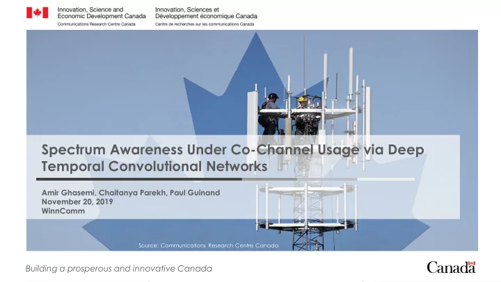
Spectrum Awareness Under Co-Channel Usage via Deep Temporal Convolutional Networks

Amir Ghasemi, Chaitanya Parekh, Paul Guinand November 20, 2019 WinnComm

Building a prosperous and innovative Canada

Source: Communications Research Centre Canada

Overview

• Motivation
• Background
• Proposed Scheme
• Performance Analysis
• Summary and Future Work

2

Communications Research Centre Canada (CRC)

3

Government of Canada’s primary R&D lab for advanced telecommunications

4

Providing ‘just-in-time’ spectrum knowledge

50+ spectrum sensors in Canada

USRP Spectrum Explorers ISOC

Storage Processing Analytics

Cloud infrastructure

Spectrum Environment Awareness

5

• Special events
• Traffic conditions
• Weather conditions
• Financial conditions
• Ensemble user

behaviour

Predictor Modelling Sharing Policies Business & Policy Needs Spectrum Intelligence Sensors

Radio Spectrum

Spectrum Allocation & Assignment Decision Engine Predictor Data Fusion & Analytics Analysis

Making Better Use of Spectrum

Motivation

• Spectrum sharing is expected to be the norm in some bands
• Spectrum awareness is a key enabler for sharing to ensure

fairness, regulatory compliance, and avoid harmful interference

• Sensing at low signal-to-noise-ratio (SNR) and co-channel

interference is critical esp. for protection of incumbent services

6

Background – Modulation Classification

• Traditionally relying on domain experts and carefully-

crafted features

• Auto-correlation and spectral correlation functions,

cyclo-stationarity

• Statistical properties of amplitude and phase
• Features are derived and fed into conventional

classifiers (small neural nets, decision trees, SVMs, …)

7

Background

• Feature detectors require (often complex)

analytical derivations for different combinations of signal, interference, channel, and noise

• Not scalable

8

• Can we instead learn to detect co-channel

modulations directly from the raw data?

Why Deep Learning

• Deep learning (DL) proven effective in

processing raw image and speech without hand-crafted features

• DL is now available at the edge
• Trained models can be adjusted

quickly for slightly different situations (transfer learning)

9

DL-Based Modulation Classification

• Raw baseband I/Q samples can be

used directly to identify the modulation using deep CNNs1

• Variations based convolutional LSTM

improved performance further2

10

• 1. T. J. O’Shea, J. Corgan, T. C. Clancy, ”Convolutional Radio Modulation Recognition Networks,” 2016,

https://arxiv.org/pdf/1602.04105

• 2. N. E. West, T. J. O’Shea, ”Deep Architectures for Modulation Recognition,” in Proc. IEEE DySPAN 2017

Temporal Convolutional Networks (TCN)*

11

• Inspired by WaveNet architecture originally

proposed by Google DeepMind

• Fully convolutional auto-regressive network

using 1-dimensional causal convolution filters

• Dilated convolutions enable using longer

training sequences

• Residual and skip connections enable training

very deep architectures

* S. Bai, J. Z. Kolter, V. Koltun, ”An Empirical Evaluation of Generic Convolutional and Recurrent Networks for Sequence Modeling,” available online: https://arxiv.org/abs/1803.01271, April 2018.

12

Modulation Type

TCN Architecture

~ 445,000 trainable parameters

Dataset and Scenarios

13

• Created by extending the publicly available RadioML 2016.10 dataset* for co-

channel signals scenario

• Raw I/Q vectors of length 128 and 1024 samples, generated with GNU Radio
• Single Signal:
• 8 digital modulations: GFSK, CPFSK, BPSK, PAM4, QPSK, 8PSK, 16QAM, 64QAM
• SNR levels ranging from -20 to 18dB in steps of 2dB
• 5000 vectors per SNR (total of 100k examples per modulation)

* http://deepsig.io/datasets/

• Interference Signal:
• Modulation of desired signal known and fixed
• Need to identify the modulation of a potential interferer
• Of particular interest in spectrum regulation e.g. to identify unauthorized use of a

channel licensed to a specific user

• SNR fixed at 10dB, five SIR levels (-10,-5,0,5,10 dB)
• Second signal added with random phase (uniformly distributed between 0 and 2π).
• 4000 vectors per SIR (20k examples per class)
• Mixed Signal:
• 29 Classes: All pairwise combinations of 7 digital modulations (21 classes), single signal

(7 classes), noise only (1 class)

• Second signal added with random phase (uniformly distributed between 0 and 2π)
• Four SNR levels (-18,-6,6,18 dB) and five SIR levels (-10,-5,0,5,10 dB)
• 4000 vectors per SIR/SNR combination (100k I/Q vectors per class)

Dataset and Scenarios

14

• Dataset is split 80%/10%/10% for training, validation,

and final testing with early stopping of 10 epochs to avoid over-fitting

• Network is trained using Keras with Tensorflow

backend on a Tesla V100 GPU with categorical cross- entropy loss function

Performance Analysis

15

16

Performance Analysis – Single Signal

• Short-duration dataset (128-

sample I/Q vectors)

• SNR levels ranging from -20 to

18dB in steps of 2dB

• 5000 vectors per SNR (total of

100k examples per modulation)

17

Performance Analysis – Single Signal

• Long-duration dataset (1024-

sample I/Q vectors)

Performance Analysis – Interference Classifier

18

Performance Analysis – Mixed Signals

19

Confusion matrix for mixed-signal classification across the full SNR and SIR range

Performance Analysis – Mixed Signals

20

Confusion matrix for mixed-signal classification: SNR = 18dB SIR = -10dB

Performance Analysis – Mixed Signals

21

Probability distribution of true label’s rank among the predicted labels

• Top-1 accuracy: 43%
• Top-5 accuracy: 75%

Peeking into the Classifier

22

Summary

23

• Spectrum awareness is becoming increasingly important to

users and regulators

• Data-driven approaches to sensing are model-agnostic and

not limited by analytical complexities

• Deep learning can successfully learn signal features with little

to no pre-processing

• Key challenge is to synthesize/collect representative training

data

Further Work

24

• Model interpretation
• Robustness to channel impairments
• Over-the-air experiments