Spatial dependence HELSINGIN YLIOPISTO HELSINGFORS UNIVERSITET - PDF document
Spatial dependence HELSINGIN YLIOPISTO HELSINGFORS UNIVERSITET UNIVERSITY OF HELSINKI Everything is related to everything else, but nearby things are more related than distant things Spatial Data Mining This is usually true even for spatially
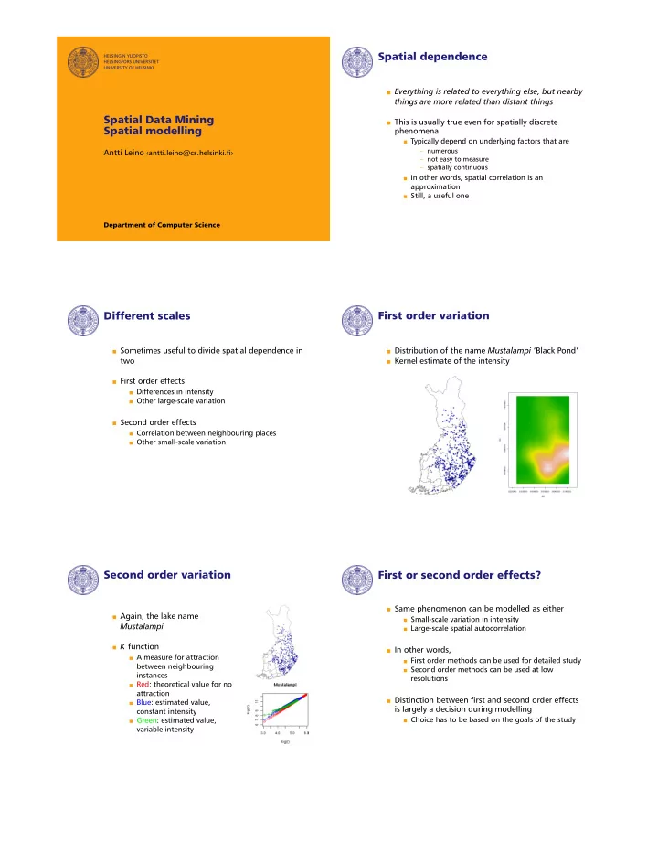
Spatial dependence HELSINGIN YLIOPISTO HELSINGFORS UNIVERSITET UNIVERSITY OF HELSINKI Everything is related to everything else, but nearby things are more related than distant things Spatial Data Mining This is usually true even for spatially discrete Spatial modelling phenomena Typically depend on underlying factors that are � numerous Antti Leino �antti.leino@cs.helsinki.�� � not easy to measure � spatially continuous In other words, spatial correlation is an approximation Still, a useful one Department of Computer Science First order variation Different scales Sometimes useful to divide spatial dependence in Distribution of the name Mustalampi 'Black Pond' two Kernel estimate of the intensity First order effects Differences in intensity Other large-scale variation Second order effects Correlation between neighbouring places Other small-scale variation Second order variation First or second order effects? Same phenomenon can be modelled as either Again, the lake name Small-scale variation in intensity Mustalampi Large-scale spatial autocorrelation K function In other words, A measure for attraction First order methods can be used for detailed study between neighbouring Second order methods can be used at low instances resolutions Red: theoretical value for no attraction Distinction between �rst and second order effects Blue: estimated value, is largely a decision during modelling constant intensity Choice has to be based on the goals of the study Green: estimated value, variable intensity
Dealing with space Background concepts No (a priori) direction Statistics commonly has certain methodological assumptions Correlations in a two-dimensional space Not reasonable to assume that correlation is Null hypothesis: the phenomenon is completely directional random Goal: prove that the null hypothesis is invalid Usually: phenomena follow the normal distribution Hence: no obvious de�nition for neighbourhood in point patterns What does this mean for spatial data? proximity in area data Complete spatial randomness Suitable probability distribution Boundary effects Observations do not typically cover all the phenomenon In reality, correlation reaches to the unseen areas This is not available for analysis Modelling spatial randomness Modelling point patterns Spatial stochastic process Randomness: the Poisson process Statistical model for a spatial phenomenon Independent events happening with a constant intensity λ Represented by the joint probability distribution of a set of random variables In its basic form one-dimensional { X ( s ), s ∈ R } for point data { Y ( A ), A ⊆ R } for area data E.g. time The probability of an event happening during an equal-sized time slot is uniform Normally only one realisation is observed The actual values of the variable in each location The expected number of events in a time slot E ( X ( t )) = λ t Poisson process: example Poisson process: example Two time sequences generated from a Poisson Probability distribution of the expected value of process with λ = 2 events A ( • ): 24 events λ = 2, t = 10 B ( ◦ ): 17 events X ( t ) ∼ Poisson ( 20 )
First order variation: intensity Poisson process: from one to two dimensions Easy to extend the Poisson process to a Instead of constant intensity λ an intensity two-dimensional case function E ( X ( d s )) λ ( s ) = lim | d s | | d s |→ 0 Again, constant intensity λ d s a neighbourhood of point s The expected number of events in region A E ( X ( d s )) the expected number of points in this depends on the intensity and the area of A : neighbourhood | d s | the size of the neighbourhood E ( X ( A )) = λ | A | The spatial Poisson process is a model of what The intensity at point s can be viewed as the would happen if the events were independent �density� of events in an in�nitely small from each other neighbourhood of s No �rst order variation No second order effects Estimating intensity Using the intensity function A Poisson process can use the intensity function Kernel estimation instead of a constant intensity Represent each point by a symmetrical two-dimensional density function, e.g. normal Such a heterogeneous Poisson process models the distribution �rst order variation of a point pattern Estimate the intensity function as the sum of these The expected number of events in a region A density functions n � 1 1 � s − s i E ( X ( A )) = λ ( s ) d s � λ τ ( s ) = τ 2 k ˆ � δ τ ( s ) A τ i = 1 s 1 ,..., s n event points k kernel function τ > 0 bandwidth δ τ ( s ) edge correction Kernel estimation Simulating a Poisson process Homogeneous Poisson process: two phases Bandwidth de�nes how far from each point the 1. Number of events in area A : n ∼ Poisson ( λ | A | effect reaches 2. The locations for the events can be obtained from a uniform distribution over A In effect, it speci�es how detailed the variation in intensity is Similarly for a heterogeneous Poisson process 1. λ not constant 2. Locations from a non-uniform distribution
Measuring second order effects K function Nearest neighbour measures Measure for second order effects G ( h ) : probability that the distance from a random event to the nearest other event ≤ h Basic case: constant λ , one point pattern F ( h ) : probability that the distance from a random λ K ( h ) = expected number of other events within location to the nearest event ≤ h radius h of a random event For a homogeneous Poisson process K ( h ) = π h 2 If events are clustered, G ( h ) < F ( h ) Also possible to measure K inhom ( h ) for a Only shows very small-scale attraction / repulsion heterogeneous point pattern Something else is required for scales larger than For two point patterns the nearest neighbour distance λ j K ij ( h ) = expected number of events of type j within radius h of a random event of type i Modelling second order variation K function: example Two pairs of lake names Poisson cluster process Mustalampi 'Black Pond' � Valkealampi 'White Pond' Start with a Poisson process Kuikkalampi 'Diver Pond' � Ruunalampi 'Gelding Normally, a homogeneous process Pond' In principle, heterogeneous also possible, but Spatial distributions and K functions dif�cult to estimate Blue line: homogeneous K ij This process generates �parents� Green line: heterogeneous K inhom ij Each parent generates a random number of �daughters� Distributed independently around the parent These are the actual events Spatially continuous phenomena First order properties of continuous data Mean value surface { µ ( s ), s ∈ R }, µ ( s ) = E ( Y ( s )) Observations from distinct points in space Normal statistical regression problem This time, measurements of a spatially continuous variable { Y ( s ), s ∈ R } Linear regression of Y ( s ) with spatial coordinates s x , s y Trend surface analysis Goal: model the behaviour of Y across R More sophisticated methods available Again, useful to divide variation into �rst and Goal: interpolate the value of Y between the second order effects observation points Y ( s ) = µ ( s )
Second order effects in continuous Predicting with second order effects data Usually better to assume Y ( s ) = µ ( s ) + U ( s ) If the residual process { U ( s ), s ∈ R } is spatially µ ( s ) global trend correlated, it is possible to give better estimates U ( s ) spatially correlated residual, with than Y ( s ) = ˆ µ ( s ) ∀ s ∈ R : E ( U ( s )) = 0 Y ( s ) = ˆ µ ( s ) + ˆ U ( s ) Kriging: ˆ U ( s ) can be used to model second order effects Various methods for this Common assumption: U ( s ) is stationary Beyond the scope of this course E ( U ( s )) and Var ( U ( s )) constant No general criterion for choosing, beyond �see Cov ( U ( s ), U ( s ′ )) depends only on h = s ′ − s what works� In other words, the same in different parts of R Bottom line: modelling both �rst and second order Often also isotropic effects gives reasonably good predictions Cov ( U ( s ), U ( s ′ )) depends only on | h | In other words, the same in all directions Proximity in area data First order variation Simple option: moving averages Proximity matrix W Replace the value for each area by the averages of its neighbours � 1 if A i and A j share a border � n w ij = j = 1 w ij y j 0 otherwise µ i = ˆ � n j = 1 w ij A B C D E F Convert to point data A 0 1 0 1 1 0 B 1 0 1 0 1 1 E.g. represent each area by its centre C 0 1 0 0 0 1 Perform kernel estimation D 1 0 0 0 1 1 E 1 1 0 1 0 1 Median polish F 0 1 1 1 1 0 For regular grids Represent each grid cell as More elaborate measures for proximity possible y ij = µ + r i + c j + ε ij r i , c j row and column trends, ε ij random error Summary Second order effects Moran's I statistic: spatial correlation Lots of statistical methods for spatial modelling n � n � n j = 1 w ij ( y i − ¯ y )( y j − ¯ y ) i = 1 Different methods for point patterns, area data I = �� n i = 1 ( y i − ¯ y ) 2 ���� i �= j w ij � and continuous data Some related to each other Varies between − 1 and + 1, no autocorrelation when I = 0 If still interested, take a course in spatial statistics Geary's C statistic: variance of the difference of neighbouring values ( n − 1 ) � n � n j = 1 w ij ( y i − y j ) 2 i = 1 C = �� n 2 i = 1 ( y i − ¯ y ) 2 ���� i �= j w ij � Varies between 0 and 2, no autocorrelation when C = 1
Recommend
More recommend
Explore More Topics
Stay informed with curated content and fresh updates.
