Spatial Birth-Death Model for Wireless Networks Abishek Sankararaman - PowerPoint PPT Presentation
Spatial Birth-Death Model for Wireless Networks Abishek Sankararaman and Franois Baccelli UT Austin Outline Motivation and Background. Math Model - Interacting Particle System. Summary of Results. Further
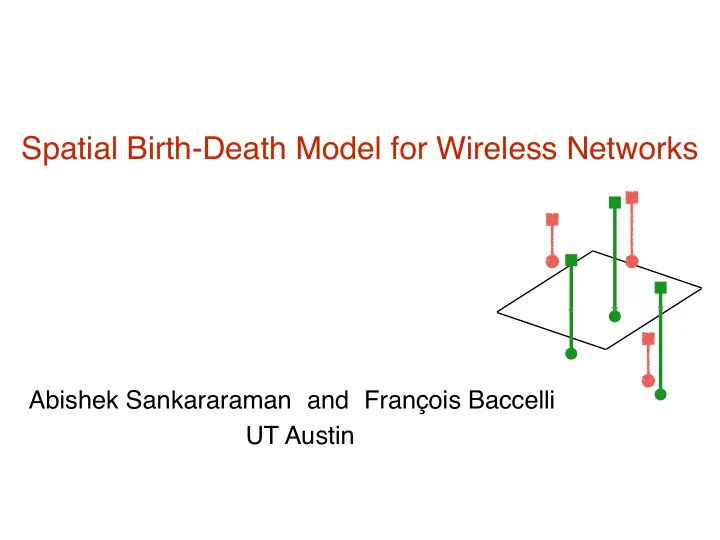
Spatial Birth-Death Model for Wireless Networks Abishek Sankararaman and François Baccelli UT Austin
Outline Motivation and Background. � • Math Model - Interacting Particle System. � • Summary of Results. � • Further Questions. •
Background and Motivation Model for a wireless network that captures precisely � • Interactions in Space � • (Interference) � � �
Background and Motivation Model for a wireless network that captures precisely � • Interactions in Space � • (Interference) � � � � Interactions in Time due to randomness in traffic. •
Background - Ad-Hoc Wireless Networks We study a simplified dynamical model for ad-hoc wireless networks. •
Background - Ad-Hoc Wireless Networks We study a simplified dynamical model for ad-hoc wireless networks. • Main engineering application - Overlaid D2D networks. • Increasing popularity of D2D as means to offload some cellular traffic. � • [Dhillon, 15], [Lee, Lin, Andrews, Heath 15], [Lu, DeVeciana 15]
Background - Ad-Hoc Wireless Networks Ad-hoc networks have been studied in detail for a long time ! •
Background - Ad-Hoc Wireless Networks Ad-hoc networks have been studied in detail for a long time ! • � However, little is understood on the spatio-temporal interactions in ad-hoc • wireless network. [Blaszczyszyn, Jovanovic, Karray `13] � � 1. Static spatial setting [Baccelli, et.al 03], [FlashLinQ 13] � (Does not precisely capture interactions through traffic arrivals) � � � 2. Flow-based queuing models (for ex. [Bonald,Proutiere 06]) � ( Does not capture precisely, the information-theoretic interactions) � �
Background - Ad-Hoc Wireless Networks Ad-hoc networks have been studied in detail for a long time ! • � However, little is understood on the spatio-temporal interactions in ad-hoc • wireless network. [Blaszczyszyn, Jovanovic, Karray `13] � � 1. Static spatial setting [Baccelli, et.al 03], [FlashLinQ 13] � (Does not precisely capture interactions through traffic arrivals) � � � 2. Flow-based queuing models (for ex. [Bonald,Proutiere 06]) � ( Does not capture precisely, the information-theoretic interactions) � � A caricature framework that captures the interactions over space and time.
Stochastic Network Model - Preliminaries
Stochastic Network Model - Preliminaries - continuum space for the network. S = [ − Q, Q ] × [ − Q, Q ] • The edges wrapped around to form a torus Links (Tx-Rx pairs) are line segments of length . • T
Stochastic Network Model - Preliminaries - continuum space for the network. S = [ − Q, Q ] × [ − Q, Q ] • The edges wrapped around to form a torus Links (Tx-Rx pairs) are line segments of length . • T λ Links arrive as a PPP on with intensity R × S • Probability of a point arriving in space and time is λ dxdt dt dx
Stochastic Network Model - Preliminaries - continuum space for the network. S = [ − Q, Q ] × [ − Q, Q ] • The edges wrapped around to form a torus Links (Tx-Rx pairs) are line segments of length . • T λ Links arrive as a PPP on with intensity R × S • Probability of a point arriving in space and time is λ dxdt dt dx Each Tx has an iid file size of mean bits to transmit to its Rx L •
Stochastic Network Model - Preliminaries - continuum space for the network. S = [ − Q, Q ] × [ − Q, Q ] • The edges wrapped around to form a torus Links (Tx-Rx pairs) are line segments of length . • T λ Links arrive as a PPP on with intensity R × S • Probability of a point arriving in space and time is λ dxdt dt dx Each Tx has an iid file size of mean bits to transmit to its Rx L • • A link exits the network after the Tx finishes transmitting its file.
Stochastic Network Model - Preliminaries - continuum space for the network. S = [ − Q, Q ] × [ − Q, Q ] • The edges wrapped around to form a torus Links (Tx-Rx pairs) are line segments of length . • T λ Links arrive as a PPP on with intensity R × S • Probability of a point arriving in space and time is λ dxdt dt dx Each Tx has an iid file size of mean bits to transmit to its Rx L • • A link exits the network after the Tx finishes transmitting its file. • : The configuration of links present in the system at time φ t t φ t = { ( x 1 , y 1 ) , ( x 2 , y 2 ) , · · · , ( x N t , y N t ) } (Configuration at time t).
Line Segment - Arrival Departure Schematic Spatial Domain S The “ “ appear as a Poisson Process φ t The green represent The red lines represent space-time � (Time = t) position of links that are either dead � by time t or not yet born at time t. Increasing Time
Basic Notation φ t • : The configuration of links present in the system at time t φ Rx = { x 1 , x 2 , · · · , x N t } The set of receivers at time t t φ T x = { y 1 , y 2 , · · · , y N t } The set of transmitters at time t t || x i − y i || = T ∀ i Tx ( x i ) = y i Note - is a random variable depending on the dynamics N t φ t = { ( x 1 , y 1 ) , ( x 2 , y 2 ) , · · · , ( x N t , y N t ) } (Configuration at time t).
Stochastic Network Model - Dynamics Links arrive in the network as a PPP on with intensity λ • R × S Each Tx has an iid exponential file size of mean bits to transmit to � L • its Rx • A point exits the network after the Tx finishes transmitting its file. Speed of file transfer ? φ t = { ( x 1 , y 1 ) , ( x 2 , y 2 ) , · · · , ( x N t , y N t ) } (Configuration at time t).
Stochastic Network Model - Dynamics Links arrive in the network as a PPP on with intensity λ • R × S Each Tx has an iid exponential file size of mean bits to transmit to � L • its Rx • A point exits the network after the Tx finishes transmitting its file. Speed of file transfer ? Given by the instantaneous Shannon Rate seen at each point. φ t = { ( x 1 , y 1 ) , ( x 2 , y 2 ) , · · · , ( x N t , y N t ) } (Configuration at time t).
Stochastic Network Model - Dynamics φ Interference seen at point due to configuration • x X I ( x, φ ) = l ( || y − x || ) (distance measured on the torus). y ∈ φ T x \ T x ( x ) l ( · ) : R + → R + called the ‘path-loss function’. y 1 φ = { ( x, Tx ( x )) , ( x 1 , y 1 ) , ( x 2 , y 2 ) , ( x 3 , y 3 ) , ( x 4 , y 4 ) } y 2 x y 4 y 3
Stochastic Network Model - Dynamics φ Interference seen at point due to configuration • x X I ( x, φ ) = l ( || y − x || ) (distance measured on the torus). y ∈ φ T x \ T x ( x ) l ( · ) : R + → R + called the ‘path-loss function’. φ Speed of file-transfer to point in configuration • x ✓ ◆ l ( T ) R ( x, φ ) = C log 2 1 + bits per second N 0 + I ( x, φ ) A deterministic function of the configuration y 1 φ = { ( x, Tx ( x )) , ( x 1 , y 1 ) , ( x 2 , y 2 ) , ( x 3 , y 3 ) , ( x 4 , y 4 ) } y 2 x y 4 y 3
Stochastic Network Model - Dynamics The speed of file transfer by link at location in configuration φ • x ✓ ◆ l ( T ) R ( x, φ ) = C log 2 1 + bits per second N 0 + I ( x, φ ) φ 1 = { ( x, Tx ( x )) , ( y 1 , Tx ( y 1 )) , ( y 2 , Tx ( y 2 )) , y 1 y 2 ( y 3 , Tx ( y 3 )) , ( y 4 , Tx ( y 4 )) } x y 4 y 3 R ( x, φ 1 ) ≥ R ( x, φ 2 ) y 1 y 2 φ 1 = { ( x, Tx ( x )) , ( y 1 , Tx ( y 1 )) , ( y 2 , Tx ( y 2 )) , ( y 3 , Tx ( y 3 )) } x y 3
The Problem Statement A link ‘born’ at location and time with file-size leaves the system b p • L p x p Z u ( ) (‘dies’) at time d p = inf u ≥ b p : R ( x p , φ t ) dt ≥ L p t = b p ✓ l ( T ) ◆ where R ( x, φ ) = C log 2 1 + N 0 + I ( x, φ ) φ t and is the set of links “alive” at time . t Spatial Birth-Death Process since - Arrivals from the Poisson Rain • Departures happen after file transfer •
Spatial Birth-Death (SBD) Model Spatial Domain S The “ “ appear as a Poisson Process φ t The green represent The red lines represent space-time � (Time = t) position of links that are either dead � by time t or not yet born at time t. Increasing Time
SBD Model - Interacting Particle System A caricature framework that accounts for spatio-temporal � interactions. The rest of the talk - present results on this model Conclude with questions on how to enrich the framework to cover different aspects and applications. y 1 φ = { ( x, Tx ( x )) , ( x 1 , y 1 ) , ( x 2 , y 2 ) , ( x 3 , y 3 ) , ( x 4 , y 4 ) } y 2 x y 4 y 3
Stochastic Network Model - Details Model Assumptions. N 0 > 0 Needed to avoid the corner case of when interference is 0. • is a compact set. • S = [ − Q, Q ] × [ − Q, Q ] Want rate to be non-zero. l ( r ) < ∞ , ∀ r > 0 • The statistical assumptions imply that is a Markov Process on the set of � φ t marked simple counting measures on the set S y 1 φ = { ( x, Tx ( x )) , ( x 1 , y 1 ) , ( x 2 , y 2 ) , ( x 3 , y 3 ) , ( x 4 , y 4 ) } y 2 x y 4 y 3
Some Comments on the Model Continuum space-time stochastic system. •
Recommend
More recommend
Explore More Topics
Stay informed with curated content and fresh updates.
