Spatial assessment of association between total fertility and under - PDF document
Spatial assessment of association between total fertility and under five mortality rate in high fertility states of India Author Akansha Singh Universite Catholique de Louvain, Belgium Email: akansha.singh@uclouvain.be Abstract Global efforts
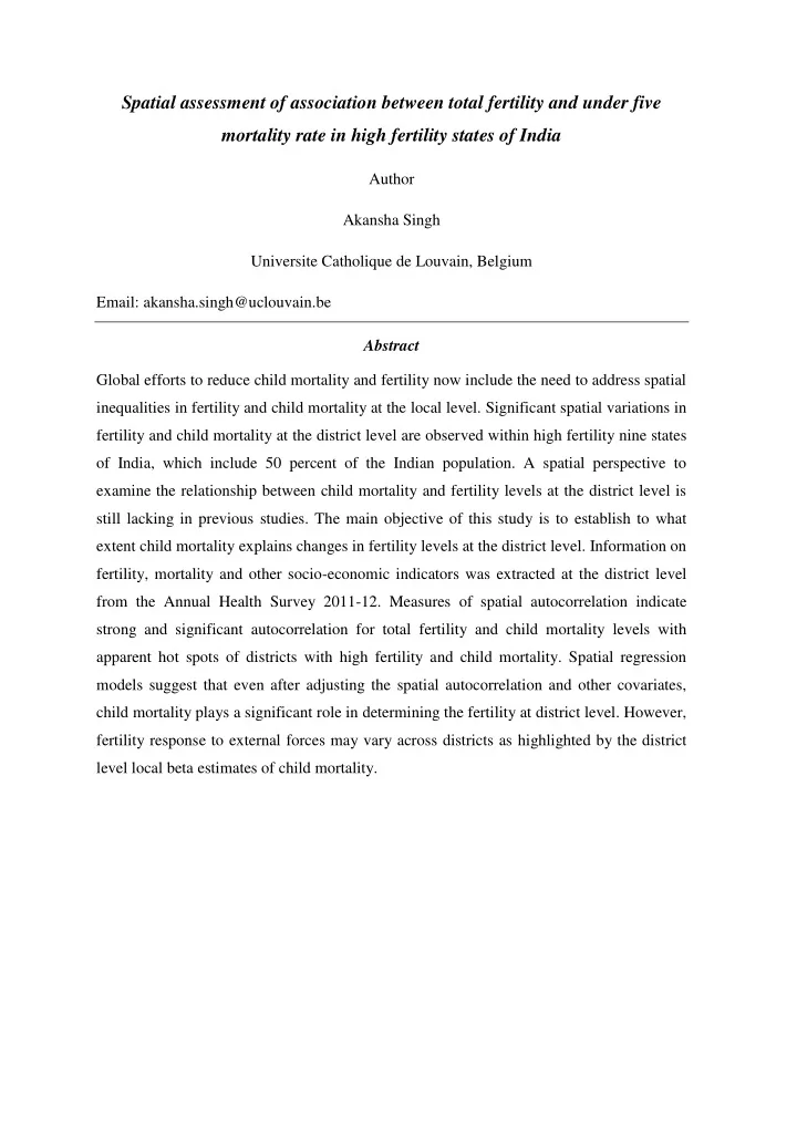
Spatial assessment of association between total fertility and under five mortality rate in high fertility states of India Author Akansha Singh Universite Catholique de Louvain, Belgium Email: akansha.singh@uclouvain.be Abstract Global efforts to reduce child mortality and fertility now include the need to address spatial inequalities in fertility and child mortality at the local level. Significant spatial variations in fertility and child mortality at the district level are observed within high fertility nine states of India, which include 50 percent of the Indian population. A spatial perspective to examine the relationship between child mortality and fertility levels at the district level is still lacking in previous studies. The main objective of this study is to establish to what extent child mortality explains changes in fertility levels at the district level. Information on fertility, mortality and other socio-economic indicators was extracted at the district level from the Annual Health Survey 2011-12. Measures of spatial autocorrelation indicate strong and significant autocorrelation for total fertility and child mortality levels with apparent hot spots of districts with high fertility and child mortality. Spatial regression models suggest that even after adjusting the spatial autocorrelation and other covariates, child mortality plays a significant role in determining the fertility at district level. However, fertility response to external forces may vary across districts as highlighted by the district level local beta estimates of child mortality.
Introduction Over the past few decades, several studies have looked into the trends, patterns and determinants of total fertility rate in India. All studies have highlighted significant regional variations in fertility behaviour in India. This has beenmainly attributed to the cultural, economic and geographical diversity in the country. Mapping fertility transition during the period 1951-1991 showed that fertility decline began in India’s periphery, along the coasts and in the extreme south. The fertility decline then spread progressively inward, gradually moving north, to encircle the region surrounding the Ganges Valley, the heart of Hindi- speaking traditional India, where fertility has hardly declined at all (Guilmoto and Rajan 2001). This region in the upper part of India is predominantly identified by high fertility and child mortality rates. Several studies have shown the north, south divide in fertility and mortality transition in India (Saikia et al., 2011; Guilmoto and Rajan 2001). Moreover, improvements in total fertility and child mortality have been uneven and the burden of high fertility and mortality is still disproportionately borne by the certain pockets of this region. These studies illustrate significant variations in fertility and child mortality at the district level within high fertility states of India (Guilmoto and Rajan 2013). These states include nine major states of India with 50 percent of the Indian population and lagging in many socioeconomic and demographic indicators. The population stabilization of India is contingent on the future fertility scenario in these states (Das and Mohanty 2012). Hence, there is huge significance of analysing fertility levels in these nine major states comprises Assam, Bihar, Chhattisgarh, Jharkhand, Madhya Pradesh, Rajasthan, Uttar Pradesh and Uttarakhand (See Figure 1). Very few studies allow the assessment of fertility levels at the district level of India. These studies have tried to examine the factors associated with fertility at district level (Guilmoto and Rajan 2001; Guilmoto and Rajan 2013; Das and Mohanty 2012). A comprehensive spatial evaluation of the fertility at the district level in high fertility states of India is missing from all such studies. Child mortality has been identified as one of the most important factor explaining the variation in fertility at the district levels (Guilmoto and Rajan 2001; Das and Mohanty 2012). However, the basic question that comes is does this relationship hold even after adjusting for spatial dependency and controlling the socio economic condition of the districts. Further, the key lies in establishing to what extent child mortality explains the change in fertility levels in the global and the local levels in high fertility surroundings of India.
The objective of this study is twofold: (1) to understand the spatial differentials in total fertility rates and the child mortality rate in India and (2) to investigate the relationship between fertility level and the child mortality at the global and local levels adjusting for other socio economic variables. Data source This study is focused on nine high focus states in India - Bihar, Chhattisgarh, Jharkhand, Madhya Pradesh, Orissa, Rajasthan, Uttarakhand, Uttar Pradesh and Assam, consisting of 284 districts. These nine states account for about 50% of the total population in the country, are the high focus states in view of their relatively high fertility and mortality indicators. The district level data of total fertility rate and under- five mortality rate for all nine states were obtained from the recently concluded Annual Health Survey (AHS) – 2011-12 (Registrar General and Census Commissioner 2015). Other socio-economic variables include the female literacy rate, female mean age at marriage, female work force participation, male work participation rate, proportion of urban population, female contraceptive prevalence rate and under five mortality rate. Table 1 provides the description of the variables used in this study. Table 1: Main outcome and independent variables in the regression analysis Variables Description Total fertility rate TFR Female literacy rate Fliterate Female mean age at marriage Fmarriage Female work participation rate FWPR Male work participation rate MWPR Proportion of urban population Urban Modern Contraceptive prevalence rate CPR Under five mortality rate U5MR Spatial analysis methods At the first state, spatial autocorrelation has been estimated to examine coincidence of value similarity with locational similarity (Anselin and Bera 1998). It can be computed at both national and local level. The former takes into account the spatial configuration of the whole area whereas the later measures spatial association of a variable at a location with that in its local neighbourhood. Computation of spatial autocorrelation requires constructing a matrix, known as spatial weights neighbourhood matrix (W), to quantify the spatial proximity for each observational unit (district). In this analysis, contiguity based weights (queen) with all first order neighbours were considered in generating the spatial
weights neighbourhood matrix. We used these weights to manifest the spatial clustering and outliers in the outcome variable (TFR) and main independent variable (U5MR) using ∗ ). Moran's I statistics and LISA (Local Indicators of Spatial Autocorrelation) ( 𝐽 𝑘 ∗ ) LISA statistic ( 𝐽 Moran's I statistic (I) 𝑘 ̅ denotes its average over all regions/ districts, N is Here Y i is indicator of interest at i th district, 𝑍 total number of regions/ districts and w ij is an element of the matrix W defined above corresponding to the pair of locations i and j A correlation matrix was computed to assess the association between the outcome variable and predictors before applying the multivariate OLS and spatial models. We have tested the spatial dependency in classical statistical models using robust lagrange multiplier error and lag test. Further based on the finding from the classical analysis we moved further to compare three regression models to examine the relationship between the outcome variable and a set of predictors: ordinary least square (OLS), spatial lag model (SLM) and spatial error model. Spatial Lag Model : If dependent variable, Y , is correlated with weighted average of its value in the neighbourhood and other locations, this relationship can be expressed as: Y = ρWY + βX + ɛ Here, ρ is spatial lag parameter, W is spa tial weights matrix, X is vector of explanatory variables and β is corresponding coefficient vector. It is assumed here that the error terms εs are identically and independently distributed (iids) although one can correct for heteroscedasticity (Anselin 2003). A significant spatial lag term may indicate strong spatial dependence. Spatial Error Model : If the spatial dependence enters the model through the error term, ε , we have the spatial error model: Y = βX + ɛ ɛ = λW ɛ + μ
Recommend
More recommend
Explore More Topics
Stay informed with curated content and fresh updates.

