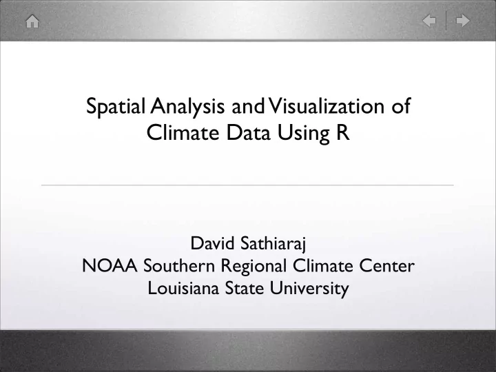
Spatial Analysis and Visualization of Climate Data Using R David - PowerPoint PPT Presentation
Spatial Analysis and Visualization of Climate Data Using R David Sathiaraj NOAA Southern Regional Climate Center Louisiana State University ACIS ACIS - Applied Climate Information System (www.rcc-acis.org) Provides Storage, Access and
Spatial Analysis and Visualization of Climate Data Using R David Sathiaraj NOAA Southern Regional Climate Center Louisiana State University
ACIS • ACIS - Applied Climate Information System (www.rcc-acis.org) • Provides Storage, Access and Analysis of Climate Data • 3 layer abstracted architecture - comprises of station meta data, climate data and derived product layers • Data Source for generating maps
QC Disk Real Time Feed Disk Disk Data Metadata Sets Data Synchronization Products
Why R? • Simple data structures • Robust matrix computations • Spatial libraries • Visualization tools
Map Generation Tools • Color Selection - RColorBrewer • Masking - sp • Map Projection - mapproj • Fitting and Modeling - fields, sp
Mapping Climate Divisions • Climate divisions shape file usdiv = readShapePoly(“divisions.shp”) )# plot(usdiv,col=brewer.pal(11, `Spectral’) (# • Get a subset of climate divisions • '# Choose Color (based on climate data) "# • Plot and Draw legend ! !"# ! !!# ! !## ! $# ! %# ! &#
Mapping Climate Divisions (" • Get a subset of climate divisions • '# Using subset command in R • Choose Color (based on climate '" data) • Plot and Draw legend &# ! !"# ! !"" ! $# ! $" ! %#
Mapping Climate Divisions • Choose Color (based on 2005 Prcp Total: SRCC Divisions climate data) (" - colours <- brewer.pal(nclr,"RdYlGn") '# - ratio<-(max(prcp)-min(prcp))/nclr )2.-./01 - brks<- round(seq(min(prcp),max(prcp), '" by=ratio),digits=0) - colorIndx <- findInterval(prcp, brks, all.inside=T) &# • Plot and Draw legend ! !"# ! !"" ! $# ! $" ! %# )*+,-./01
Mapping Climate Divisions 2005 Prcp Total: SRCC Divisions • (" Plot and Draw legend - plot(srccdiv_shp, col=colours[colorIndx], '# xlab="Longitude", ylab="Latitude") )2.-./01 - '" title("2005 Prcp Total: SRCC /+0134!% Divisions") !%4 ! 4&' &'4 ! 4&$ &$4 ! 4'( '(4 ! 4(" - ("4 ! 4(# legend(-87.5, 30, (#4 ! 4#" #"4 ! 4#5 &# legend=leglabs(brks), *6134#5 fill=colours, cex=1, bty="o") ! !"# ! !"" ! $# ! $" ! %# )*+,-./01
2005 Prcp Total: SRCC Divisions (" '# )2.-./01 '" /+0134!% !%4 ! 4&' &'4 ! 4&$ &$4 ! 4'( '(4 ! 4(" ("4 ! 4(# (#4 ! 4#" #"4 ! 4#5 &# *6134#5 ! !"# ! !"" ! $# ! $" ! %# )*+,-./01
Surface Fitting • Fields package in R • krig.image (from fields) • tim.colors (from fields) • Masking Routine • Map projection
Kriging using fields fit=krig.image(xy,z,cov.function=Exp.image.cov,m=mx,n=nx,lambda=0.01, kmax=1000,expand=1.2) res<- predict( fit, fit$xM) - fit$yM img=list(fit$surface$x,fit$surface$y,fit$surface$z) proj_pts = mapproject(list(x=img$x,y=img$y),projection="mercator") proj_img = list(x=proj_pts$x,y=proj_pts$y,z=img$z) proj_img = mask(proj_img) image.plot(proj_img,col=rev(tim.colors(64)),xlab='Longitude',ylab='La titude',add=1,projection="",horizontal=1)
Masking • Pass the array of fitted points to the masking routine • Find which points lie ‘inside’ the polygon(I) and which lie ‘outside’ (O) - ‘inout’ method in the ‘sp’ package • Nullify the ‘outside’ points, O • one possibility is assign their ‘z’ values to NA • Return the array comprising of nullified outside points, O and ‘inside’ points, I
● ● ● ● ● ● ● ● ● ● ● ● ● ● ● ● ● 37 ● ● ● ● ● ● ● ● ● ● ● ● ● ● ● ● ● ● ● ● ● ● ● ● ● ● ● ● ● ● ● ● ● ● ● ● ● ● 36 ● ● ● ● ● ● ● ● ● ● ● ● ● ● ● ● ● ● ● ● ● ● ● ● ● ● ● ● ● ● ● ● ● ● ● ● ● ● ● Latitude 35 ● ● ● ● ● ● ● ● ● ● ● ● ● ● ● ● ● ● ● ● ● ● ● ● ● ● ● ● ● ● ● ● ● ● ● ● ● ● ● ● ● ● ● ● ● ● ● ● ● ● ● ● ● ● ● ● ● ● 34 ● ● ● ● ● ● ● ● ● ● ● ● ● ● ● ● ● ● ● ● ● ● ● ● ● ● ● ● ● ● ● ● ● ● ● ● ● ● ● ● ● 33 ● ● ● ● ● ● ● ● ● ● ● ● ● ● ● ● ● ● ● ● ● ● ● ● ● ● ● ● ● ● ● ● ● ● ● ● ● ● ● ● ● ● ● ● ● ● 32 ● − 95 − 94 − 93 − 92 − 91 − 90 − 89 Longitude
Charts using R Baton Rouge Ryan Airport 100 90 80 Temperature [F] 70 60 50 40 30 01 15 01 15 01 15 01 15 01 15 01 15 01 15 01 15 01 15 01 15 01 15 01 15 Jan Feb Mar Apr May Jun Jul Aug Sep Oct Nov Dec 60 50 Precipitation [in] 40 30 20 10 0 01 15 01 15 01 15 01 15 01 15 01 15 01 15 01 15 01 15 01 15 01 15 01 15 Jan Feb Mar Apr May Jun Jul Aug Sep Oct Nov Dec 2007
Recommend
More recommend
Explore More Topics
Stay informed with curated content and fresh updates.
