sous-titres du masque 6th WMO Symposium on DA Washington DC - 2013 - PowerPoint PPT Presentation

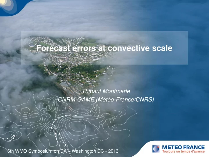
Forecast errors at convective scale Cliquez pour modifier le style du titre Thibaut Montmerle Cliquez pour modifier le style des CNRM-GAME (Météo-France/CNRS) sous-titres du masque 6th WMO Symposium on DA – Washington DC - 2013

Outlines  Context: NWP at convective scale Forecast errors at convective scale:  Specific features compared to global scale  B modelling - climatological formulation - adding flow dependencies (- hydrometeors)  B deduced from ensembles  Conclusions

Context: NWP at convective scale Non-hydrostatic models (in the 1-3 km horizontal resolution range) allow realistic representation of convection, clouds, precipitation, turbulence, surface interactions Specific features: • Need coupling models to provide LBCs and surface conditions • Observations linked to clouds and precipitation can be considered (e.g radars) • Analyses must be performed frequently • Forecasts are very Radar reflectivity simulated by expensive in computation AROME time!!

Context: NWP at convective scale The AROME NWP system (Seity et al. 2011) • Oper since more than 5 years, dx=2.5 km, LBCs provided by ARPEGE • Same observations than ARPEGE with radar DOW and reflectivities Surface Sat IASI TEMP ~1.3 10 8 variables Aircraft DA based on « real time » RADAR RH ensembles unaffordable for the time RADAR being DOW Active obs in AROME for one rainy day

Outlines  Context: NWP at convective scale Forecast errors at convective scale:  Specific features compared to global scale  B modelling - climatological formulation - adding flow dependencies  B deduced from ensembles  Conclusions

Specific features compared to Global scale Use of an EDA based on AROME with 90 members to produce a background perturbations database e k 2 )) o Fisher 2003 ; Kucukkaraca and Fisher (2006); Berre et al 2006

Specific features compared to Global scale B can be approximated using N background perturbations: N å ( ) ( ) 1 T B = x k - x x k - x N - 1 k = 1 B = V 1/2 CV T /2 B B can be split in variances / correlations: V • Variances are the diagonal terms of • Correlations can be approximated locally using the tensor of the Local Correlation Hessian (LCH, Weaver and Mirouze (2012)) : ( ) r = 0 H = - ÑÑ T c r • H is computed using the covariances of normalized perturbation derivatives (Michel 2012) • Local correlation lengths are then deduced in the direction of the eigen vectors of H using its eigen values: b = l g ( ) - 1/2 H L g

Background error variances for q at 945 hPa : Ménétrier et al. 2013 AEARO 90: convective scale AEARP 90: global scale • Some features are clearly specific to convective scale processes and are reflecting the resolution differences (e.g uncertainty of low level convergence, orographic precipitations…) • Low correlations for all variables (not shown) Downscaling from global models seems not Radar adapted

Total L b and ellipses of the LCH tensor (=> correlation shapes around the origin) for q at 945 hPa For AROME: • Much shorter length-scales, much more anisotropic structures • Small values over mountains and in precipitations • Correlation function elongated along the meridional flow over Med. • Large scale perturbations advected inside the domain due to coupling Ménétrier et al. 2013

Outlines  Context: NWP at convective scale Forecast errors at convective scale:  Specific features compared to global scale  B modelling - climatological formulation - adding flow dependencies  B deduced from ensembles  Conclusions

B modelling An operational NWP system at convective scale : • generally uses 3DVar with frequent assimilation/forecast steps to avoid the TL/AD coding of strongly non-linear parameterizations (e.g diabatic processes) and to benefit from observations with high temporal resolutions • uses a sequence of sparse operators to model B , that can not be expressed at full rank (~(10 8 ) 2 ) • is commonly based on an incremental formulation with CVT transform d x = B C 1/2 c 1/2 the known important The challenge is to capture in B c features of B

B modelling 1/2 = K P B S 1/2 : Typical structure of B c B C 1/2 (Derber and Bouttier (1999)  K p : Balance operators (or parameter transform) that decorrelate multivariate relationships  B S 1/2 : Spatial transforms that decorrelate univariate unbalanced variables + variance scaling Assumes that errors in balanced variables are uncorrelated from errors in unbalanced variables Typically transforms to variables which are assumed to be uncorrelated Such formulation allows to get balanced analyzed fields These operators are calibrated using ensemble of forecast differences to get climatological static values

B modelling Balance operator in AROME: • Computed for spectral fields with an extra relationship for q ( ) u + d q u (Berre 2000) d q = QH dz + R dh u + S d T , d P S • Analytical linear balance to ensure geostrophical balance • Use of regression operators that adjust couplings with scales => the latter balance can be relaxed for smaller scales Balance operator at the Met-Office (similar to WRF, CMC..) • fields in spatial representation instead of spectral • analytical operators instead of statistical regressions (incl. NLBE, hydrostatic balance (that may be invalid at CS)) (More details can be found in Bannister (2008))

B modelling Known limitations of climatological balance operators Strong dependencies to weather type (Brousseau et al, 2011) and to meteorological phenomena that are under-represented in the ensemble Often high impact weather! Normalized deviation from linear geostrophical balance for Clim Rain different types of rain (Carron and Fillion (2010)) Total (T,Ps) u Unbalanced divergence Mass field balanced with vorticity Also, deviation from hydrostatic Fraction of explained variance ratios for q balance (Vetra-Carvalho et al. 2012) (Montmerle and Berre (2010))

B modelling Improvement of climatological balance operators in deterministic VAR For the larger scales (Fisher, 2003): • NLBE • Quasi-Geostrophic omega and continuity equations A diabatic forcing of balanced vertical motion, as diagnosed by Pagé et al. (2007) could (hardly) be introduced in the latter Use of the heterogeneous formulation with M geographical masks(Ménétrier and Montmerle (2011) for fog, Montmerle (2012) for precipitation): M å B C = T /2 F 1/2 B C i F i i i = 1 Where F i defines the area where the ad-hoc B ci is applied

B modelling B S = S C S T Spatial transforms : diagonal matrix of stationary grid-point b In areas of high uncertainties (often high impact weather!), error variances are under-estimated: the analysis is not sufficiently corrected C : - vertical correlations represented by empirical functions (e.g EOFs) - horizontal correlations usually computed using the diagonal spectral hypothesis (bi-Fourier series for AROME), or in grid-point space by using recursive filters (Purser et al, 2003) (WRF, JMA…) The resulting correlations are homogeneous and isotropic

B modelling Spatial transform Again, strong dependencies to the meteorological phenomena of the horizontal correlation length-scales and of the vertical auto-correlations Example for fog: Oper Fog No fog Vertical autocorrelations for T (zoom in the first 200m 500m) Ménétrier and Montmerle (2011)

B modelling Adding anisotropies in spatial transforms • Different length-scales corresponding to different meteorological phenomena can be imposed in specific areas using the heterogeneous VAR formulation (Montmerle and Berre, 2010) in e.g precipitating regions • Wavelet formulation allows to model simultaneously scale and position-dependent aspects of covariances (Fisher, 2003) • Covariances can be streched in recursive filters (Purser et al., 2003b) • Isotropic correlations can be computed in an objectively distorted grid (Michel 2012) •…

B modelling Mesoscale Horizontal correlations modelized by wavelets (Deckmyn and Berre (2005)) B wavelets Raw correlations

B modelling Grid deformation for horizontal error correlations (Michel 2012) Distorted grid (where Raw correlations are homogeneous and isotropic) Back to regular grid Modeled diagonal spectral

B modelling Deformation of vertical error correlations Adaptative mesh transform for vertical correlations that uses a monitor function that depends on the static stability d /dz from the guess (Piccolo and Cullen (2012)) Mesh points are concentrated around T inversions or cloud top height Vertical cross sections of monitor function (top) and of the corresponding adaptative mesh (bottom)

B modelling Use of optimally filtered error variances from small ensemble Adaptation of Raynaud et. al (2009) work at convective scale (See B. Ménétrier poster (B-p13) ) • Tests are ongoing to modulate B C by such Optimally Filtered error variances Raw • Potentially useful in an EnVAR context: Oper complementary to localization as it allows to reduce the sampling noise locally 2 for q u RMSE of averaged b

Outlines  Context: NWP at convective scale Forecast errors at convective scale:  Specific features compared to global scale  B modelling - climatological formulation - adding flow dependencies  B deduced from ensembles  Conclusions