Sorting & Master Theorem CS16: Introduction to Data Structures - PowerPoint PPT Presentation

Sorting & Master Theorem CS16: Introduction to Data Structures & Algorithms Spring 2020

Outline ‣ Motivation ‣ Quadratic Sorting ‣ Selection sort ‣ Insertion sort ‣ Linearithmic Sorting ‣ Merge Sort ‣ Master Theorem ‣ Quick Sort ‣ Comparative sorting lower bound ‣ Linear Sorting ‣ Radix Sort

The Problem ‣ Turn this 10 19 7 4 3 21 10 23 24 18 1 8 23 1 12 ‣ Into this 1 1 3 4 7 8 10 10 12 18 19 21 23 23 24 ‣ as efficiently as possible 3

Sorting is Serious! 4

Sorting Competition ‣ Sort Benchmark (sortbenchmark.org) ‣ Started by Jim Gray ‣ Research scientist at Microsoft Research ‣ Winner of 1998 Turing Award for contributions to databases ‣ Tencent Sort from Tencent Corp. (2016) ‣ 100 TB in 134 seconds ‣ 37 TB in 1 minute 5

Why? ‣ Why do we care so much about sorting? ‣ Rule of thumb: ‣ “good things happen when data is sorted” ‣ we can find things faster (e.g., using binary search) 6

Sorting Algorithms ‣ There are many ways to sort arrays ‣ Iterative vs. recursive ‣ in-place vs. not-in-place ‣ comparison-based vs. non-comparative ‣ In-place algorithms ‣ transform data structure w/ small amount of extra storage (i.e., O(1) ) ‣ For sorting: array is overwritten by output instead of creating new array ‣ Most sorting algorithms in 16 are comparison-based ‣ main operation is comparison ‣ but not all (e.g., Radix sort) 7

“In-Placeness” ‣ Reversing an array function reverse (A): function reverse (A): n = A.length n = A.length B = array of length n for i = 0 to n/2: for i = 0 to n – 1: temp = A[i] B[n − 1 − i] = A[i] A[i] = A[n − 1 − i] return B A[n − 1 − i] = temp in-place Not in-place! Return statement not needed 8

Properties of In-Place Solutions ‣ Harder to write :-( ‣ Use less memory :-) ‣ Even harder to write for recursive algorithms :-( ‣ Tradeoff between simplicity an efficiency 9

Outline ‣ Motivation ‣ Quadratic Sorting ‣ Selection sort ‣ Insertion sort ‣ Linearithmic Sorting ‣ Merge Sort ‣ Master Theorem ‣ Quick Sort ‣ Comparative sorting lower bound ‣ Linear Sorting ‣ Radix Sort

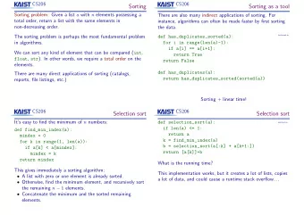
Selection Sort ‣ Usually iterative and in-place ‣ Divides input array into two logical parts ‣ elements already sorted ‣ elements that still need to be sorted ‣ Selects smallest element & places it at index 0 ‣ then selects second smallest & places it in index 1 ‣ then the third smallest at index 2 , etc.. 11

Selection Sort ‣ Advantages ‣ Very simple ‣ Memory efficient if in-place (swaps elements in array) ‣ Disadvantages ‣ Slow: O(n 2 ) 12

Selection Sort ‣ Iterate through positions min 53 25 13 22 9 ‣ At each position 9 25 13 22 53 ‣ store smallest element from remaining set min 9 13 25 22 53 min 9 13 22 25 53 min 9 13 22 25 53

Selection Sort function selection_sort (A): n = A.length for i = 0 to n-2: min = argmin(A[i:n-1]) swap A[i] with A[min] 14

Outline ‣ Motivation ‣ Quadratic Sorting ‣ Selection sort ‣ Insertion sort ‣ Linearithmic Sorting ‣ Merge Sort ‣ Master Theorem ‣ Quick Sort ‣ Comparative sorting lower bound ‣ Linear Sorting ‣ Radix Sort

Insertion Sort ‣ Usually iterative and in-place ‣ Compares each item w/ all items before it… ‣ …and inserts it into correct position ‣ Advantages ‣ Works really well if items partially sorted ‣ Memory efficient if in-place (swaps elements in array) ‣ Disadvantages ‣ Slow: O(n 2 ) 16

Insertion Sort ‣ Compares each item w/ all items before it… 53 25 13 22 23 ‣ …and inserts it into correct position 25 53 13 22 23 13 25 53 22 23 Note: 23 > 22 so don’t need to 13 22 25 53 23 keep checking since rest is already sorted 13 22 23 25 53

Insertion Sort function insertion_sort (A): n = A.length for i = 1 to n-1: for j = i down to 1: if a[j] < a[j-1]: swap a[j] and a[j-1] else: break # out of the inner for loop # this prevents double checking the 
 # already sorted portion 18

Outline ‣ Motivation ‣ Quadratic Sorting ‣ Selection sort ‣ Insertion sort ‣ Linearithmic Sorting ‣ Merge Sort ‣ Master Theorem ‣ Quick Sort ‣ Comparative sorting lower bound ‣ Linear Sorting ‣ Radix Sort

Divide & Conquer ‣ Algorithmic design paradigm ‣ divide: divide input S into disjoint subsets S 1 ,…,S k ‣ recur: solve sub-problems on S 1 ,…,S k ‣ conquer: combine solutions for S 1 ,…,S k into solution for S ‣ Base case is usually sub-problem of size 1 or 0 20

Merge Sort ‣ Sorting algorithm based on divide & conquer ‣ Like quadratic sorts ‣ comparative ‣ Unlike quadratic sorts ‣ recursive ‣ linearithmic O(nlog n) 21

Merge Sort ‣ Merge sort on n-element sequence S ‣ divide: divide S into disjoint subsets S 1 and S 2 ‣ recur: recursively merge sort S 1 and S 2 ‣ conquer: merge S 1 and S 2 into sorted sequence ‣ Suppose we want to sort ‣ 7,2,9,4,3,8,6,1 22

Merge Sort Recursion Tree ➞ 1 2 3 4 6 7 8 9 7 2 9 4 3 8 6 1 ➞ 2 7 4 9 7 2 9 4 ➞ 1 3 6 8 3 8 6 1 6 1 ➞ 1 6 3 8 ➞ 3 8 ➞ 4 9 7 2 ➞ 2 7 9 4 ➞ ➞ ➞ ➞ 9 4 ➞ ➞ 7 9 4 8 ➞ ➞ 7 2 2 3 8 3 6 1 6 1 23

Merge Sort Pseudo-Code function mergeSort (A): if A.length <= 1: return A mid = A.length/2 left = mergeSort(A[0...mid-1]) right = mergeSort(A[mid...n-1]) return merge(left, right) 24

Merge Sort Pseudo-Code function merge (A, B): result = [] aIndex = 0 bIndex = 0 while aIndex < A.length and bIndex < B.length: if A[aIndex] <= B[bIndex]: result.append(A[aIndex]) aIndex++ else: result.append(B[bIndex]) bIndex++ if aIndex < A.length: result = result + A[aIndex:end] if bIndex < B.length: result = result + B[bIndex:end] return result 25

Merge Sort 2 min Activity #1 26

Merge Sort 2 min Activity #1 27

Merge Sort 1 min Activity #1 28

Merge Sort 0 min Activity #1 29

Merge Sort Recurrence Relation ‣ Merge sort steps ‣ Recursively merge sort left half ‣ Recursively merge sort right half ‣ Merge both halves ‣ T(n) : time to merge sort input of size n ‣ T(n) = step 1 + step 2 + step 3 ‣ Steps 1 & 2 are merge sort on half input so T(n/2) ‣ Step 3 is O(n) 30

Merge Sort Recurrence Relation ‣ General case ⇣ n ⇣ n ⇣ n ⌘ ⌘ ⌘ T ( n ) = T + T + O ( n ) = 2 · T + O ( n ) 2 2 2 ‣ Base case T (1) = c 31

Merge Sort Recurrence Relation ‣ Plug & chug T (1) = c 1 T (2) = 2 · T (1) + 2 = 2 c 1 + 2 T (4) = 2 · T (2) + 4 = 2(2 c 1 + 2)4 = 4 c 1 + 8 T (8) = 2 · T (4) + 8 = 2(4 c 1 + 8) + 8 = 8 c 1 + 24 T (16) = 2 · T (8) + 16 = 2(8 c 1 + 24) + 16 = 16 c 1 + 64 ‣ Solution T ( n ) = nc 1 + n log n = O ( n log n ) 32

Analysis of Merge Sort ‣ Merge sort recursive tree is perfect binary tree so has height O(log n) ‣ At each depth k : need to merge 2 k+1 sequences of size n/2 k+1 ‣ work at each depth is O(n) depth sequenc size es 0 2 n/2 1 4 n/4 2 8 n/4 ⋮ ⋮ ⋮ … … … … � � � � k 2 k+1 n/2 k+1 33

Analysis of Merge Sort ‣ To determine that Merge sort was O(nlog n) ‣ Use plug and chug to guess a solution ‣ Prove that O(n log n) is correct (e.g., using induction) ‣ Can be a lot of work 34

Outline ‣ Motivation ‣ Quadratic Sorting ‣ Selection sort ‣ Insertion sort ‣ Linearithmic Sorting ‣ Merge Sort ‣ Master Theorem ‣ Quick Sort ‣ Comparative sorting lower bound ‣ Linear Sorting ‣ Radix Sort

36

The Master Theorem ‣ Solves large class of recurrence relations ‣ we will learn how to use it but not its proof ‣ See Dasgupta et al. p. 58-60 for proof ‣ Let T(n) be a monotonically-increasing function of form ⇣ n ⌘ + Θ ( n d ) T ( n ) = a · T b ‣ a : number of sub-problems ‣ n/b : size of each sub-problem ‣ n d : work to prepare sub-problems & combine their solutions 37

The Master Theorem ‣ If a ≥ 1 , b>1 , d ≥ 0 , then ‣ if a<b d then T(n) = Θ (n d ) ‣ if a=b d then T(n) = Θ (n d log n) ‣ if a>b d then T(n) = Θ (n logba ) ‣ Applying Master Theorem to merge sort ‣ Recurrence relation of merger sort: T(n) = 2T(n/2)+O(n 1 ) ‣ a=2 , b=2 and d=1 so a=b d ‣ and T(n) = Θ (n d log n) 
 = Θ (n 1 log n) 
 = Θ (n log n) 38

Master Theorem ⇣ n ⌘ + Θ ( n d ) T ( n ) = a · T b ‣ T(n) = Θ (n d ) if a<b d ‣ T(n) = Θ (n d log n) if a=b d ‣ T(n) = Θ (n logba ) if a>b d 2 min Activity #2+3 39

Master Theorem ⇣ n ⌘ + Θ ( n d ) T ( n ) = a · T b ‣ T(n) = Θ (n d ) if a<b d ‣ T(n) = Θ (n d log n) if a=b d ‣ T(n) = Θ (n logba ) if a>b d 2 min Activity #2+3 40

Master Theorem ⇣ n ⌘ + Θ ( n d ) T ( n ) = a · T b ‣ T(n) = Θ (n d ) if a<b d ‣ T(n) = Θ (n d log n) if a=b d ‣ T(n) = Θ (n logba ) if a>b d 1 min Activity #2+3 41

Master Theorem ⇣ n ⌘ + Θ ( n d ) T ( n ) = a · T b ‣ T(n) = Θ (n d ) if a<b d ‣ T(n) = Θ (n d log n) if a=b d ‣ T(n) = Θ (n logba ) if a>b d 0 min Activity #2+3 42

Outline ‣ Motivation ‣ Quadratic Sorting ‣ Selection sort ‣ Insertion sort ‣ Linearithmic Sorting ‣ Merge Sort ‣ Master Theorem ‣ Quick Sort ‣ Comparative sorting lower bound ‣ Linear Sorting ‣ Radix Sort